Agent-based models

This HTML version of Think Complexity, 2nd Edition is provided for convenience, but it is not the best format of the book. In particular, some of the symbols are not rendered correctly.

Chapter 9 Agent-based models

The models we have seen so far might be characterized as “rule-based” in the sense that they involve systems governed by simple rules. In this and the following chapters, we explore agent-based models.

Agent-based models include agents that are intended to model people and other entities that gather information about the world, make decisions, and take actions.

The agents are usually situated in space or in a network, and interact with each other locally. They usually have imperfect or incomplete information about the world.

Often there are differences among agents, unlike previous models where all components are identical. And agent-based models often include randomness, either among the agents or in the world.

Since the 1970s, agent-based modeling has become an important tool in economics, other social sciences, and some natural sciences.

Agent-based models are useful for modeling the dynamics of systems that are not in equilibrium (although they are also used to study equilibrium). And they are particularly useful for understanding relationships between individual decisions and system behavior.

The code for this chapter is in chap09.ipynb, which is a Jupyter notebook in the repository for this book. For more information about working with this code, see Section ??.

9.1 Schelling’s Model

In 1969 Thomas Schelling published “Models of Segregation”, which proposed a simple model of racial segregation. You can read it at http://thinkcomplex.com/schell.

The Schelling model of the world is a grid where each cell represents a house. The houses are occupied by two kinds of agents, labeled red and blue, in roughly equal numbers. About 10% of the houses are empty.

At any point in time, an agent might be happy or unhappy, depending on the other agents in the neighborhood, where the “neighborhood" of each house is the set of eight adjacent cells. In one version of the model, agents are happy if they have at least two neighbors like themselves, and unhappy if they have one or zero.

The simulation proceeds by choosing an agent at random and checking to see whether they are happy. If so, nothing happens; if not, the agent chooses one of the unoccupied cells at random and moves.

You will not be surprised to hear that this model leads to some segregation, but you might be surprised by the degree. From a random starting point, clusters of similar agents form almost immediately. The clusters grow and coalesce over time until there are a small number of large clusters and most agents live in homogeneous neighborhoods.

If you did not know the process and only saw the result, you might assume that the agents were racist, but in fact all of them would be perfectly happy in a mixed neighborhood. Since they prefer not to be greatly outnumbered, they might be considered mildly xenophobic. Of course, these agents are a wild simplification of real people, so it may not be appropriate to apply these descriptions at all.

Racism is a complex human problem; it is hard to imagine that such a simple model could shed light on it. But in fact it provides a strong argument about the relationship between a system and its parts: if you observe segregation in a real city, you cannot conclude that individual racism is the immediate cause, or even that the people in the city are racists.

Of course, we have to keep in mind the limitations of this argument: Schelling’s model demonstrates a possible cause of segregation, but says nothing about actual causes.

9.2 Implementation of Schelling’s model

To implement Schelling’s model, I wrote yet another class that inherits from Cell2D:

n is the size of the grid, and p is the threshold on the fraction of similar neighbors. For example, if p=0.3, an agent will be unhappy if fewer than 30% of their neighbors are the same color.

array is a NumPy array where each cell is 0 if empty, 1 if occupied by a red agent, and 2 if occupied by a blue agent. Initially 10% of the cells are empty, 45% red, and 45% blue.

The step function for Schelling’s model is substantially more complicated than previous examples. If you are not interested in the details, you can skip to the next section. But if you stick around, you might pick up some NumPy tips.

First, I make boolean arrays that indicate which cells are red, blue, and empty:

Then I use correlate2d to count, for each location, the number of neighboring cells that are red, blue, and non-empty. We saw correlate2d in Section ??.

options is a dictionary that contains the options we pass to correlate2d. With mode='same', the result is the same size as the input. With boundary='wrap', the top edge is wrapped to meet the bottom, and the left edge is wrapped to meet the right.

kernel indicates that we want to consider the eight neighbors that surround each cell.

After computing num_red and num_blue, we can compute the fraction of neighbors, for each location, that are red and blue.

Then, we can compute the fraction of neighbors, for each agent, that are the same color as the agent. I use np.where, which is like an element-wise if expression. The first parameter is a condition that selects elements from the second or third parameter.

In this case, wherever red is True, frac_same gets the corresponding element of frac_red. Where red is False, frac_same gets the corresponding element of frac_blue. Finally, where empty indicates that a cell is empty, frac_same is set to np.nan, which is a special value that indicates “Not a Number”.

np.nonzero takes an array and returns the coordinates of all non-zero cells; the result is a tuple of arrays, one for each dimension. Then locs_where uses list and zip to convert this result to a list of coordinate pairs.

Similarly, empty_locs is an array that contains the coordinates of the empty cells:

Now we get to the core of the simulation. We loop through the unhappy agents and move them:

i is the index of a random empty cell; dest is a tuple containing the coordinates of the empty cell.

In order to move an agent, we copy its value (1 or 2) from source to dest, and then set the value of source to 0 (since it is now empty).

Finally, we replace the entry in empty_locs with source, so the cell that just became empty can be chosen by the next agent.

9.3 Segregation

Now let’s see what happens when we run the model. I’ll start with n=100 and p=0.3, and run for 10 steps.

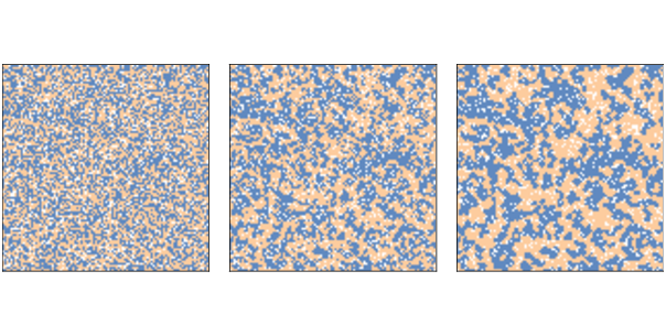
Figure ?? shows the initial configuration (left), the state of the simulation after 2 steps (middle), and the state after 10 steps (right).

Clusters form almost immediately and grow quickly, until most agents live in highly-segregated neighborhoods.

As the simulation runs, we can compute the degree of segregation, which is the average, across agents, of the fraction of neighbors who are the same color as the agent:

In Figure ??, the average fraction of similar neighbors is 50% in the initial configuration, 65% after two steps, and 76% after 10 steps!

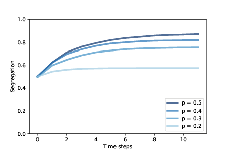
Remember that when p=0.3 the agents would be happy if 3 of 8 neighbors were their own color, but they end up living in neighborhoods where 6 or 7 of their neighbors are their own color, typically.

Figure ?? shows how the degree of segregation increases and where it levels off for several values of p. When p=0.4, the degree of segregation in steady state is about 82%, and a majority of agents have no neighbors with a different color.

These results are surprising to many people, and they make a striking example of the unpredictable relationship between individual decisions and system behavior.

9.4 Sugarscape

In 1996 Joshua Epstein and Robert Axtell proposed Sugarscape, an agent-based model of an “artificial society” intended to support experiments related to economics and other social sciences.

Sugarscape is a versatile model that has been adapted for a wide variety of topics. As examples, I will replicate the first few experiments from Epstein and Axtell’s book, Growing Artificial Societies.

In its simplest form, Sugarscape is a model of a simple economy where agents move around on a 2-D grid, harvesting and accumulating “sugar”, which represents economic wealth. Some parts of the grid produce more sugar than others, and some agents are better at finding it than others.

This version of Sugarscape is often used to explore and explain the distribution of wealth, in particular the tendency toward inequality.

In the Sugarscape grid, each cell has a capacity, which is the maximum amount of sugar it can hold. In the original configuration, there are two high-sugar regions, with capacity 4, surrounded by concentric rings with capacities 3, 2, and 1.

Figure ?? (left) shows the initial configuration, with the darker areas indicating cells with higher capacity, and small dots representing the agents.

Initially there are 400 agents placed at random locations. Each agent has three randomly-chosen attributes:

During each time step, agents move one at a time in a random order. Each agent follows these rules:

After all agents have executed these steps, the cells grow back some sugar, typically 1 unit, but the total sugar in each cell is bounded by its capacity.

Figure ?? (middle) shows the state of the model after two steps. Most agents are moving toward the areas with the most sugar. Agents with high vision move the fastest; agents with low vision tend to get stuck on the plateaus, wandering randomly until they get close enough to see the next level.

Agents born in the areas with the least sugar are likely to starve unless they have a high initial endowment and high vision.

Within the high-sugar areas, agents compete with each other to find and harvest sugar as it grows back. Agents with high metabolism or low vision are the most likely to starve.

When sugar grows back at 1 unit per time step, there is not enough sugar to sustain the 400 agents we started with. The population drops quickly at first, then more slowly, and levels off around 250.

Figure ?? (right) shows the state of the model after 100 time steps, with about 250 agents. The agents who survive tend to be the lucky ones, born with high vision and/or low metabolism. Having survived to this point, they are likely to survive forever, accumulating unbounded stockpiles of sugar.

9.5 Wealth inequality

In its current form, Sugarscape models a simple ecology, and could be used to explore the relationship between the parameters of the model, like the growth rate and the attributes of the agents, and the carrying capacity of the system (the number of agents that survive in steady state). And it models a form of natural selection, where agents with higher “fitness” are more likely to survive.

The model also demonstrates a kind of wealth inequality, with some agents accumulating sugar faster than others. But it would be hard to say anything specific about the distribution of wealth because it is not “stationary”; that is, the distribution changes over time and does not reach a steady state.

However, if we give the agents finite lifespans, the model produces a stationary distribution of wealth. Then we can run experiments to see what effect the parameters and rules have on this distribution.

In this version of the model, agents have an age that gets incremented each time step, and a random lifespan chosen from a uniform distribution between 60 to 100. If an agent’s age exceeds its lifespan, it dies.

When an agent dies, from starvation or old age, it is replaced by a new agent with random attributes, so the number of agents is constant.

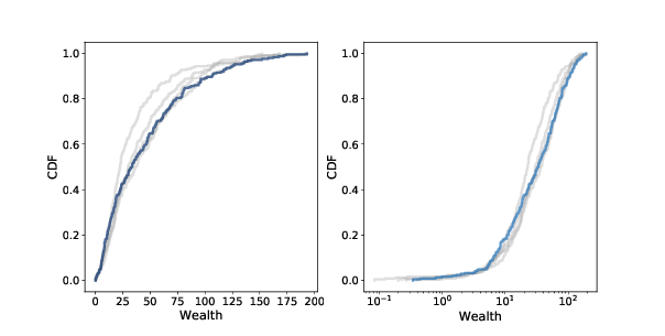
Starting with 250 agents (which is close to carrying capacity) I run the model for 500 steps. After each 100 steps, I plot the cumulative distribution function (CDF) of sugar accumulated by the agents. We saw CDFs in Section ??. Figure ?? shows the results on a linear scale (left) and a log-x scale (right).

After about 200 steps (which is twice the longest lifespan) the distribution doesn’t change much. And it is skewed to the right.

Most agents have little accumulated wealth: the 25th percentile is about 10 and the median is about 20. But a few agents have accumulated much more: the 75th percentile is about 40, and the highest value is more than 150.

On a log scale the shape of the distribution resembles a Gaussian or normal distribution, although the right tail is truncated. If it were actually normal on a log scale, the distribution would be lognormal, which is a heavy-tailed distribution. And in fact, the distribution of wealth in practically every country, and in the world, is a heavy-tailed distribution.

It would be too much to claim that Sugarscape explains why wealth distributions are heavy-tailed, but the prevalence of inequality in variations of Sugarscape suggests that inequality is characteristic of many economies, even very simple ones. And experiments with rules that model taxation and other income transfers suggest that it is not easy to avoid or mitigate.

9.6 Implementing Sugarscape

Sugarscape is more complicated than the previous models, so I won’t present the entire implementation here. I will outline the structure of the code and you can see the details in the Jupyter notebook for this chapter, chap09.ipynb, which is in the repository for this book. If you are not interested in the details, you can skip this section.

During each step, the agent moves, harvests sugar, and ages. Here is the Agent class and its step method:

The parameter env is a reference to the environment, which is a Sugarscape object. It provides methods look_and_move and harvest:

Sugarscape inherits from Cell2D, so it is similar to the other grid-based models we’ve seen.

The attributes include agents, which is a list of Agent objects, and occupied, which is a set of tuples, where each tuple contains the coordinates of a cell occupied by an agent.

During each step, the Sugarscape uses the NumPy function permutation so it loops through the agents in random order. It invokes step on each agent and then checks whether it is dead. After all agents have moved, some of the sugar grows back. The return value is the number of agents still alive.

I won’t show more details here; you can see them in the notebook for this chapter. If you want to learn more about NumPy, you might want to look at these functions in particular:

9.7 Migration and Wave Behavior

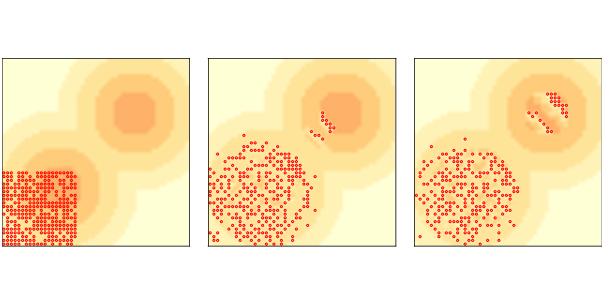
Although the purpose of Sugarscape is not primarily to explore the movement of agents in space, Epstein and Axtell observed some interesting patterns when agents migrate.

If we start with all agents in the lower-left corner, they quickly move toward the closest “peak” of high-capacity cells. But if there are more agents than a single peak can support, they quickly exhaust the sugar and agents are forced to move into lower-capacity areas.

The ones with the longest vision cross the valley between the peaks and propagate toward the northeast in a pattern that resembles a wave front. Because they leave a stripe of empty cells behind them, other agents don’t follow until the sugar grows back.

The result is a series of discrete waves of migration, where each wave resembles a coherent object, like the spaceships we saw in the Rule 110 CA and Game of Life (see Section ?? and Section ??).

Figure ?? shows the initial condition (left) and the state of the model after 6 steps (middle) and 12 steps (right). You can see the first two waves reaching and moving through the second peak, leaving a stripe of empty cells behind. You can see an animated version of this model, where the wave patterns are more clearly visible, in the notebook for this chapter.

These waves move diagonally, which is surprising because the agents themselves only move north or east, never northeast. Outcomes like this — groups or “aggregates” with properties and behaviors that the agents don’t have — are common in agent-based models. We will see more examples in the next chapter.

9.8 Emergence

The examples in this chapter demonstrate one of the most important ideas in complexity science: emergence. An emergent property is a characteristic of a system that results from the interaction of its components, not from their properties.

To clarify what emergence is, it helps to consider what it isn’t. For example, a brick wall is hard because bricks and mortar are hard, so that’s not an emergent property. As another example, some rigid structures are built from flexible components, so that seems like a kind of emergence. But it is at best a weak kind, because structural properties follow from well understood laws of mechanics.

In contrast, the segregation we see in Schelling’s model is an emergent property because it is not caused by racist agents. Even when the agents are only mildly xenophobic, the outcome of the system is substantially different from the intention of the agent’s decisions.

The distribution of wealth in Sugarscape might be an emergent property, but it is a weak example because we could reasonably predict it based on the distributions of vision, metabolism, and lifespan. The wave behavior we saw in the last example might be a stronger example, since the wave displays a capability — diagonal movement — that the agents do not have.

Emergent properties are surprising: it is hard to predict the behavior of the system even if we know all the rules. That difficulty is not an accident; in fact, it may be the defining characteristic of emergence.

As Wolfram discusses in A New Kind of Science, conventional science is based on the axiom that if you know the rules that govern a system, you can predict its behavior. What we call “laws” are often computational shortcuts that allow us to predict the outcome of a system without building or observing it.

But many cellular automatons are computationally irreducible, which means that there are no shortcuts. The only way to get the outcome is to implement the system.

The same may be true of complex systems in general. For physical systems with more than a few components, there is usually no model that yields an analytic solution. Numerical methods provide a kind of computational shortcut, but there is still a qualitative difference.

Analytic solutions often provide a constant-time algorithm for prediction; that is, the run time of the computation does not depend on t, the time scale of prediction. But numerical methods, simulation, analog computation, and similar methods take time proportional to t. And for many systems, there is a bound on t beyond which we can’t compute reliable predictions at all.

These observations suggest that emergent properties are fundamentally unpredictable, and that for complex systems we should not expect to find natural laws in the form of computational shortcuts.

To some people, “emergence” is another name for ignorance; by this reckoning, a property is emergent if we don’t have a reductionist explanation for it, but if we come to understand it better in the future, it would no longer be emergent.

The status of emergent properties is a topic of debate, so it is appropriate to be skeptical. When we see an apparently emergent property, we should not assume that there can never be a reductionist explanation. But neither should we assume that there has to be one.

The examples in this book and the principle of computational equivalence give good reasons to believe that at least some emergent properties can never be “explained” by a classical reductionist model.

9.9 Exercises

The code for this chapter is in the Jupyter notebook chap09.ipynb in the repository for this book. Open this notebook, read the code, and run the cells. You can use this notebook to work on the following exercises. My solutions are in chap09soln.ipynb.

Exercise 1

Bill Bishop, author of The Big Sort, argues that American society is increasingly segregated by political opinion, as people choose to live among like-minded neighbors.

The mechanism Bishop hypothesizes is not that people, like the agents in Schelling’s model, are more likely to move if they are isolated, but that when they move for any reason, they are likely to choose a neighborhood with people like themselves.

Modify your implementation of Schelling’s model to simulate this kind of behavior and see if it yields similar degrees of segregation.

There are several ways you can model Bishop’s hypothesis. In my implementation, a random selection of agents moves during each step. Each agent considers k randomly-chosen empty locations and chooses the one with the highest fraction of similar neighbors. How does the degree of segregation depend on k?

Exercise 2

In the first version of SugarScape, we never add agents, so once the population falls, it never recovers. In the second version, we only replace agents when they die, so the population is constant. Now let’s see what happens if we add some “population pressure”.

Write a version of SugarScape that adds a new agent at the end of every step. Add code to compute the average vision and the average metabolism of the agents at the end of each step. Run the model for a few hundred steps and plot the population over time, as well as the average vision and average metabolism.

You should be able to implement this model by inheriting from SugarScape and overriding __init__ and step.

Exercise 3

Among people who study philosophy of mind, “Strong AI" is the theory that an appropriately-programmed computer could have a mind in the same sense that humans have minds.

John Searle presented a thought experiment called “The Chinese Room”, intended to show that Strong AI is false. You can read about it at http://thinkcomplex.com/searle.

What is the system reply to the Chinese Room argument? How does what you have learned about emergence influence your reaction to the system response?