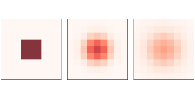
This HTML version of Think Complexity, 2nd Edition is provided for convenience, but it is not the best format of the book. In particular, some of the symbols are not rendered correctly.

You might prefer to read the PDF version.

Chapter 7 Physical modeling

The cellular automatons we have seen so far are not physical models; that is, they are not intended to describe systems in the real world. But some CAs are intended as physical models.

In this chapter we consider a CA that models chemicals that diffuse (spread out) and react with each other, which is a process Alan Turing proposed to explain how some animal patterns develop.

And we’ll experiment with a CA that models percolation of liquid through porous material, like water through coffee grounds. This model is the first of several models that exhibit phase change behavior and fractal geometry, and I’ll explain what both of those mean.

The code for this chapter is in chap07.ipynb in the repository for this book. More information about working with the code is in Section ??.

7.1 Diffusion

In 1952 Alan Turing published a paper called “The chemical basis of morphogenesis”, which describes the behavior of systems involving two chemicals that diffuse in space and react with each other. He showed that these systems produce a wide range of patterns, depending on the diffusion and reaction rates, and conjectured that systems like this might be an important mechanism in biological growth processes, particularly the development of animal coloration patterns.

Turing’s model is based on differential equations, but it can be implemented using a cellular automaton.

Before we get to Turing’s model, we’ll start with something simpler: a diffusion system with just one chemical. We’ll use a 2-D CA where the state of each cell is a continuous quantity (usually between 0 and 1) that represents the concentration of the chemical.

We’ll model the diffusion process by comparing each cell with the average of its neighbors. If the concentration of the center cell exceeds the neighborhood average, the chemical flows from the center to the neighbors. If the concentration of the center cell is lower, the chemical flows the other way.

The following kernel computes the difference between each cell and the average of its neighbors:

kernel = np.array([[0, 1, 0], [1,-4, 1], [0, 1, 0]])

Using np.correlate2d, we can apply this kernel to each cell in an array:

c = correlate2d(array, kernel, mode='same')

We’ll use a diffusion constant, r, that relates the difference in concentration to the rate of flow:

array += r * c

Figure 7.1: A simple diffusion model after 0, 5, and 10 steps.

Figure ?? shows results for a CA with size n=9, diffusion constant r=0.1, and initial concentration 0 everywhere except for an “island” in the middle. The figure shows the starting configuration and the state of the CA after 5 and 10 steps. The chemical spreads from the center outward, continuing until the concentration is the same everywhere.

7.2 Reaction-diffusion

Now let’s add a second chemical. I’ll define a new object, ReactionDiffusion, that contains two arrays, one for each chemical:

class ReactionDiffusion(Cell2D): def __init__(self, n, m, params, noise=0.1): self.params = params self.array = np.ones((n, m), dtype=float) self.array2 = noise * np.random.random((n, m)) add_island(self.array2)

n and m are the number of rows and columns in the array. params is a tuple of parameters, which I explain below.

array represents the concentration of the first chemical, A; the NumPy function ones initializes it to 1 everywhere. The data type float indicates that the elements of A are floating-point values.

array2 represents the concentration of B, which is initialized with random values between 0 and noise, which is 0.1 by default. Then add_island adds an island of higher concentration in the middle:

def add_island(a, height=0.1): n, m = a.shape radius = min(n, m) // 20 i = n//2 j = m//2 a[i-radius:i+radius, j-radius:j+radius] += height

The radius of the island is one twentieth of n or m, whichever is smaller. The height of the island is height, with the default value 0.1.

Here is the step function that updates the arrays:

def step(self): A = self.array B = self.array2 ra, rb, f, k = self.params cA = correlate2d(A, self.kernel, **self.options) cB = correlate2d(B, self.kernel, **self.options) reaction = A * B**2 self.array += ra * cA - reaction + f * (1-A) self.array2 += rb * cB + reaction - (f+k) * B

The parameters are

ra:: The diffusion rate of A (analogous to r in the previous section).
rb:: The diffusion rate of B. In most versions of this model, rb is about half of ra.
f:: The “feed” rate, which controls how quickly A is added to the system.
k:: The “kill” rate, which controls how quickly B is removed from the system.

Now let’s look more closely at the update statements:

reaction = A * B**2 self.array += ra * cA - reaction + f * (1-A) self.array2 += rb * cB + reaction - (f+k) * B

The arrays cA and cB are the result of applying a diffusion kernel to A and B. Multiplying by ra and rb yields the rate of diffusion into or out of each cell.

The term A * B**2 represents the rate that A and B react with each other. Assuming that the reaction consumes A and produces B, we subtract this term in the first equation and add it in the second.

The term f * (1-A) determines the rate that A is added to the system. Where A is near 0, the maximum feed rate is f. Where A approaches 1, the feed rate drops off to zero.

Finally, the term (f+k) * B determines the rate that B is removed from the system. As B approaches 0, this rate goes to zero.

As long as the rate parameters are not too high, the values of A and B usually stay between 0 and 1.

Figure 7.2: Reaction-diffusion model with parameters f=0.035 and k=0.057 after 1000, 2000, and 4000 steps.

With different parameters, this model can produce patterns similar to the stripes and spots on a variety of animals. In some cases, the similarity is striking, especially when the feed and kill parameters vary in space.

For all simulations in this section, ra=0.5 and rb=0.25.

Figure ?? shows results with f=0.035 and k=0.057, with the concentration of B shown in darker colors. With these parameters, the system evolves toward a stable configuration with light spots of A on a dark background of B.

Figure 7.3: Reaction-diffusion model with parameters f=0.055 and k=0.062 after 1000, 2000, and 4000 steps.

Figure ?? shows results with f=0.055 and k=0.062, which yields a coral-like pattern of B on a background of A.

Figure 7.4: A reaction-diffusion model with parameters f=0.039 and k=0.065 after 1000, 2000, and 4000 steps.

Figure ?? shows results with f=0.039 and k=0.065. These parameters produce spots of B that grow and divide in a process that resembles mitosis, ending with a stable pattern of equally-spaced spots.

Since 1952, observations and experiments have provided some support for Turing’s conjecture. At this point it seems likely, but not yet proven, that many animal patterns are actually formed by reaction-diffusion processes of some kind.

7.3 Percolation

Percolation is a process in which a fluid flows through a semi-porous material. Examples include oil in rock formations, water in paper, and hydrogen gas in micropores. Percolation models are also used to study systems that are not literally percolation, including epidemics and networks of electrical resistors. See http://thinkcomplex.com/perc.

Percolation models are often represented using random graphs like the ones we saw in Chapter ??, but they can also be represented using cellular automatons. In the next few sections we’ll explore a 2-D CA that simulates percolation.

In this model:

Initially, each cell is either “porous” with probability q or “non-porous” with probability 1-q.
When the simulation begins, all cells are considered “dry” except the top row, which is “wet”.
During each time step, if a porous cell has at least one wet neighbor, it becomes wet. Non-porous cells stay dry.
The simulation runs until it reaches a “fixed point” where no more cells change state.

If there is a path of wet cells from the top to the bottom row, we say that the CA has a “percolating cluster”.

Two questions of interest regarding percolation are (1) the probability that a random array contains a percolating cluster, and (2) how that probability depends on q. These questions might remind you of Section ??, where we considered the probability that a random Erdős-Rényi graph is connected. We will see several connections between that model and this one.

I define a new class to represent a percolation model:

class Percolation(Cell2D): def __init__(self, n, q): self.q = q self.array = np.random.choice([1, 0], (n, n), p=[q, 1-q]) self.array[0] = 5

n and m are the number of rows and columns in the CA.

The state of the CA is stored in array, which is initialized using np.random.choice to choose 1 (porous) with probability q, and 0 (non-porous) with probability 1-q.

The state of the top row is set to 5, which represents a wet cell. Using 5, rather than the more obvious 2, makes it possible to use correlate2d to check whether any porous cell has a wet neighbor. Here is the kernel:

kernel = np.array([[0, 1, 0], [1, 0, 1], [0, 1, 0]])

This kernel defines a 4-cell “von Neumann” neighborhood; unlike the Moore neighborhood we saw in Section ??, it does not include the diagonals.

This kernel adds up the states of the neighbors. If any of them are wet, the result will exceed 5. Otherwise the maximum result is 4 (if all neighbors happen to be porous).

We can use this logic to write a simple, fast step function:

def step(self): a = self.array c = correlate2d(a, self.kernel, mode='same') self.array[(a==1) & (c>=5)] = 5

This function identifies porous cells, where a==1, that have at least one wet neighbor, where c>=5, and sets their state to 5, which indicates that they are wet.

Figure 7.5: The first three steps of a percolation model with n=10 and p=0.7.

Figure ?? shows the first few steps of a percolation model with n=10 and p=0.7. Non-porous cells are white, porous cells are lightly shaded, and wet cells are dark.

7.4 Phase change

Now let’s test whether a random array contains a percolating cluster:

def test_perc(perc): num_wet = perc.num_wet() while True: perc.step() if perc.bottom_row_wet(): return True new_num_wet = perc.num_wet() if new_num_wet == num_wet: return False num_wet = new_num_wet

test_perc takes a Percolation object as a parameter. Each time through the loop, it advances the CA one time step. It checks the bottom row to see if any cells are wet; if so, it returns True, to indicate that there is a percolating cluster.

During each time step, it also computes the number of wet cells and checks whether the number increased since the last step. If not, we have reached a fixed point without finding a percolating cluster, so test_perc returns False.

To estimate the probability of a percolating cluster, we generate many random arrays and test them:

def estimate_prob_percolating(n=100, q=0.5, iters=100): t = [test_perc(Percolation(n, q)) for i in range(iters)] return np.mean(t)

estimate_prob_percolating makes 100 Percolation objects with the given values of n and q and calls test_perc to see how many of them have a percolating cluster. The return value is the fraction that do.

When p=0.55, the probability of a percolating cluster is near 0. At p=0.60, it is about 70%, and at p=0.65 it is near 1. This rapid transition suggests that there is a critical value of p near 0.6.

We can estimate the critical value more precisely using a random walk. Starting from an initial value of q, we construct a Percolation object and check whether it has a percolating cluster. If so, q is probably too high, so we decrease it. If not, q is probably too low, so we increase it.

Here’s the code:

def find_critical(n=100, q=0.6, iters=100): qs = [q] for i in range(iters): perc = Percolation(n, q) if test_perc(perc): q -= 0.005 else: q += 0.005 qs.append(q) return qs

The result is a list of values for q. We can estimate the critical value, q_crit, by computing the mean of this list. With n=100 the mean of qs is about 0.59; this value does not seem to depend on n.

The rapid change in behavior near the critical value is called a phase change by analogy with phase changes in physical systems, like the way water changes from liquid to solid at its freezing point.

A wide variety of systems display a common set of behaviors and characteristics when they are at or near a critical point. These behaviors are known collectively as critical phenomena. In the next section, we explore one of them: fractal geometry.

7.5 Fractals

To understand fractals, we have to start with dimensions.

For simple geometric objects, dimension is defined in terms of scaling behavior. For example, if the side of a square has length l, its area is l². The exponent, 2, indicates that a square is two-dimensional. Similarly, if the side of a cube has length l, its volume is l³, which indicates that a cube is three-dimensional.

More generally, we can estimate the dimension of an object by measuring some kind of size (like area or volume) as a function of some kind of linear measure (like the length of a side).

As an example, I’ll estimate the dimension of a 1-D cellular automaton by measuring its area (total number of “on” cells) as a function of the number of rows.

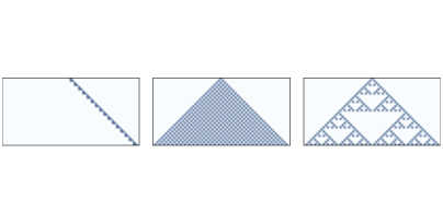
Figure 7.6: One-dimensional CAs with rules 20, 50, and 18, after 32 time steps.

Figure ?? shows three 1-D CAs like the ones we saw in Section ??. Rule 20 (left) generates a set of cells that seems like a line, so we expect it to be one-dimensional. Rule 50 (center) produces something like a triangle, so we expect it to be 2-D. Rule 18 (right) also produces something like a triangle, but the density is not uniform, so its scaling behavior is not obvious.

I’ll estimate the dimension of these CAs with the following function, which counts the number of on cells after each time step. It returns a list of tuples, where each tuple contains i, i², and the total number of cells.

def count_cells(rule, n=500): ca = Cell1D(rule, n) ca.start_single() res = [] for i in range(1, n): cells = np.sum(ca.array) res.append((i, i**2, cells)) ca.step() return res

Figure 7.7: Number of “on” cells versus number of time steps for rules 20, 50, and 18.

Figure ?? shows the results plotted on a log-log scale.

In each figure, the top dashed line shows y = i². Taking the log of both sides, we have logy = 2 logi. Since the figure is on a log-log scale, the slope of this line is 2.

Similarly, the bottom dashed line shows y = i. On a log-log scale, the slope of this line is 1.

Rule 20 (left) produces 3 cells every 2 time steps, so the total number of cells after i steps is y = 1.5 i. Taking the log of both sides, we have logy = log1.5 + logi, so on a log-log scale, we expect a line with slope 1. In fact, the estimated slope of the line is 1.01.

Rule 50 (center) produces i+1 new cells during the ith time step, so the total number of cells after i steps is y = i² + i. If we ignore the second term and take the log of both sides, we have logy ∼ 2 logi, so as i gets large, we expect to see a line with slope 2. In fact, the estimated slope is 1.97.

Finally, for Rule 18 (right), the estimated slope is about 1.57, which is clearly not 1, 2, or any other integer. This suggests that the pattern generated by Rule 18 has a “fractional dimension”; that is, it is a fractal.

This way of estimating a fractal dimension is called box-counting. For more about it, see http://thinkcomplex.com/box.

7.6 Fractals and Percolation Models

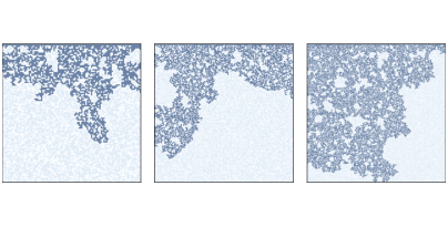
Figure 7.8: Percolation models with q=0.6 and n=100, 200, and 300.

Now let’s get back to percolation models. Figure ?? shows clusters of wet cells in percolation simulations with p=0.6 and n=100, 200, and 300. Informally, they resemble fractal patterns seen in nature and in mathematical models.

To estimate their fractal dimension, we can run CAs with a range of sizes, count the number of wet cells in each percolating cluster, and then see how the cell counts scale as we increase the size of the array.

The following loop runs the simulations:

res = [] for size in sizes: perc = Percolation(size, q) if test_perc(perc): num_filled = perc.num_wet() - size res.append((size, size**2, num_filled))

The result is a list of tuples where each tuple contains size, size**2, and the number of cells in the percolating cluster (not including the initial wet cells in the top row).

Figure 7.9: Number of cells in the percolating cluster versus CA size.

Figure ?? shows the results for a range of sizes from 10 to 100. The dots show the number of cells in each percolating cluster. The slope of a line fitted to these dots is often near 1.85, which suggests that the percolating cluster is, in fact, fractal when q is near the critical value.

When q is larger than the critical value, nearly every porous cell gets filled, so the number of wet cells is close to q * size^2, which has dimension 2.

When q is substantially smaller than the critical value, the number of wet cells is proportional to the linear size of the array, so it has dimension 1.

7.7 Exercises

Exercise 1

In Section ?? we showed that the Rule 18 CA produces a fractal. Can you find other 1-D CAs that produce fractals?

Note: the Cell1D object does not wrap around from the left edge to the right, which creates artifacts at the boundaries for some rules. You might want to use Wrap1D, which is a child class of Cell1D that wraps around. It is defined in Cell1D.py in the repository for this book.

Exercise 2

In 1990 Bak, Chen and Tang proposed a cellular automaton that is an abstract model of a forest fire. Each cell is in one of three states: empty, occupied by a tree, or on fire.

The rules of the CA are:

An empty cell becomes occupied with probability p.
A cell with a tree burns if any of its neighbors is on fire.
A cell with a tree spontaneously burns, with probability f, even if none of its neighbors is on fire.
A cell with a burning tree becomes an empty cell in the next time step.

Write a program that implements this model. You might want to inherit from Cell2D. Typical values for the parameters are p=0.01 and f=0.001, but you might want to experiment with other values.

Starting from a random initial condition, run the model until it reaches a steady state where the number of trees no longer increases or decreases consistently.

In steady state, is the geometry of the forest fractal? What is its fractal dimension?

Buy this book at Amazon.com

Contribute

If you would like to make a contribution to support my books, you can use the button below and pay with PayPal. Thank you!

Are you using one of our books in a class?

We'd like to know about it. Please consider filling out this short survey.