


This HTML version of "Think Stats 2e" is provided for convenience, but it is not the best format for the book. In particular, some of the math symbols are not rendered correctly.
You might prefer to read the PDF version, or you can buy a hard copy from Amazon.
Chapter 9 Hypothesis testing
The code for this chapter is in hypothesis.py. For information
about downloading and working with this code, see Section ??.
9.1 Classical hypothesis testing
Exploring the data from the NSFG, we saw several “apparent effects,” including differences between first babies and others. So far we have taken these effects at face value; in this chapter, we put them to the test.
The fundamental question we want to address is whether the effects we see in a sample are likely to appear in the larger population. For example, in the NSFG sample we see a difference in mean pregnancy length for first babies and others. We would like to know if that effect reflects a real difference for women in the U.S., or if it might appear in the sample by chance.
There are several ways we could formulate this question, including Fisher null hypothesis testing, Neyman-Pearson decision theory, and Bayesian inference1. What I present here is a subset of all three that makes up most of what people use in practice, which I will call classical hypothesis testing.
The goal of classical hypothesis testing is to answer the question, “Given a sample and an apparent effect, what is the probability of seeing such an effect by chance?” Here’s how we answer that question:
- The first step is to quantify the size of the apparent effect by choosing a test statistic. In the NSFG example, the apparent effect is a difference in pregnancy length between first babies and others, so a natural choice for the test statistic is the difference in means between the two groups.
- The second step is to define a null hypothesis, which is a model of the system based on the assumption that the apparent effect is not real. In the NSFG example the null hypothesis is that there is no difference between first babies and others; that is, that pregnancy lengths for both groups have the same distribution.
- The third step is to compute a p-value, which is the probability of seeing the apparent effect if the null hypothesis is true. In the NSFG example, we would compute the actual difference in means, then compute the probability of seeing a difference as big, or bigger, under the null hypothesis.
- The last step is to interpret the result. If the p-value is low, the effect is said to be statistically significant, which means that it is unlikely to have occurred by chance. In that case we infer that the effect is more likely to appear in the larger population.
The logic of this process is similar to a proof by contradiction. To prove a mathematical statement, A, you assume temporarily that A is false. If that assumption leads to a contradiction, you conclude that A must actually be true.
Similarly, to test a hypothesis like, “This effect is real,” we assume, temporarily, that it is not. That’s the null hypothesis. Based on that assumption, we compute the probability of the apparent effect. That’s the p-value. If the p-value is low, we conclude that the null hypothesis is unlikely to be true.
9.2 HypothesisTest
thinkstats2 provides HypothesisTest, a
class that represents the structure of a classical hypothesis
test. Here is the definition:
class HypothesisTest(object):

    def __init__(self, data):
        self.data = data
        self.MakeModel()
        self.actual = self.TestStatistic(data)

    def PValue(self, iters=1000):
        self.test_stats = [self.TestStatistic(self.RunModel())
                           for _ in range(iters)]

        count = sum(1 for x in self.test_stats if x >= self.actual)
        return count / iters

    def TestStatistic(self, data):
        raise UnimplementedMethodException()

    def MakeModel(self):
        pass

    def RunModel(self):
        raise UnimplementedMethodException()
HypothesisTest is an abstract parent class that provides
complete definitions for some methods and place-keepers for others.
Child classes based on HypothesisTest inherit __init__
and PValue and provide TestStatistic,
RunModel, and optionally MakeModel.
__init__ takes the data in whatever form is appropriate. It
calls MakeModel, which builds a representation of the null
hypothesis, then passes the data to TestStatistic, which
computes the size of the effect in the sample.
PValue computes the probability of the apparent effect under
the null hypothesis. It takes as a parameter iters, which is
the number of simulations to run. The first line generates simulated
data, computes test statistics, and stores them in
test_stats.
The result is
the fraction of elements in test_stats that
exceed or equal the observed test statistic, self.actual.
As a simple example2, suppose we toss a coin 250 times and see 140 heads and 110 tails. Based on this result, we might suspect that the coin is biased; that is, more likely to land heads. To test this hypothesis, we compute the probability of seeing such a difference if the coin is actually fair:
class CoinTest(thinkstats2.HypothesisTest):

    def TestStatistic(self, data):
        heads, tails = data
        test_stat = abs(heads - tails)
        return test_stat

    def RunModel(self):
        heads, tails = self.data
        n = heads + tails
        sample = [random.choice('HT') for _ in range(n)]
        hist = thinkstats2.Hist(sample)
        data = hist['H'], hist['T']
        return data
The parameter, data, is a pair of
integers: the number of heads and tails. The test statistic is
the absolute difference between them, so self.actual
is 30.
RunModel simulates coin tosses assuming that the coin is
actually fair. It generates a sample of 250 tosses, uses Hist
to count the number of heads and tails, and returns a pair of
integers.
Now all we have to do is instantiate CoinTest and call
PValue:
    ct = CoinTest((140, 110))
    pvalue = ct.PValue()
The result is about 0.07, which means that if the coin is fair, we expect to see a difference as big as 30 about 7% of the time.
How should we interpret this result? By convention, 5% is the threshold of statistical significance. If the p-value is less than 5%, the effect is considered significant; otherwise it is not.
But the choice of 5% is arbitrary, and (as we will see later) the p-value depends on the choice of the test statistics and the model of the null hypothesis. So p-values should not be considered precise measurements.
I recommend interpreting p-values according to their order of magnitude: if the p-value is less than 1%, the effect is unlikely to be due to chance; if it is greater than 10%, the effect can plausibly be explained by chance. P-values between 1% and 10% should be considered borderline. So in this example I conclude that the data do not provide strong evidence that the coin is biased or not.
9.3 Testing a difference in means
One of the most common effects to test is a difference in mean between two groups. In the NSFG data, we saw that the mean pregnancy length for first babies is slightly longer, and the mean birth weight is slightly smaller. Now we will see if those effects are statistically significant.
For these examples, the null hypothesis is that the distributions for the two groups are the same. One way to model the null hypothesis is by permutation; that is, we can take values for first babies and others and shuffle them, treating the two groups as one big group:
class DiffMeansPermute(thinkstats2.HypothesisTest):

    def TestStatistic(self, data):
        group1, group2 = data
        test_stat = abs(group1.mean() - group2.mean())
        return test_stat

    def MakeModel(self):
        group1, group2 = self.data
        self.n, self.m = len(group1), len(group2)
        self.pool = np.hstack((group1, group2))

    def RunModel(self):
        np.random.shuffle(self.pool)
        data = self.pool[:self.n], self.pool[self.n:]
        return data
data is a pair of sequences, one for each
group. The test statistic is the absolute difference in the means.
MakeModel records the sizes of the groups, n and
m, and combines the groups into one NumPy
array, self.pool.
RunModel simulates the null hypothesis by shuffling the
pooled values and splitting them into two groups with sizes n
and m. As always, the return value from RunModel has
the same format as the observed data.
To test the difference in pregnancy length, we run:
    live, firsts, others = first.MakeFrames()
    data = firsts.prglngth.values, others.prglngth.values
    ht = DiffMeansPermute(data)
    pvalue = ht.PValue()
MakeFrames reads the NSFG data and returns DataFrames
representing all live births, first babies, and others.
We extract pregnancy lengths as NumPy arrays, pass them as
data to DiffMeansPermute, and compute the p-value. The
result is about 0.17, which means that we expect to see a difference
as big as the observed effect about 17% of the time. So
this effect is not statistically significant.
Figure 9.1: CDF of difference in mean pregnancy length under the null hypothesis.
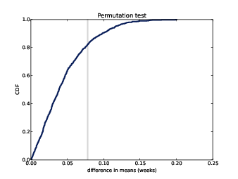
HypothesisTest provides PlotCdf, which plots the
distribution of the test statistic and a gray line indicating
the observed effect size:
    ht.PlotCdf()
    thinkplot.Show(xlabel='test statistic',
                   ylabel='CDF')
Figure ?? shows the result. The CDF intersects the observed difference at 0.83, which is the complement of the p-value, 0.17.
If we run the same analysis with birth weight, the computed p-value is 0; after 1000 attempts, the simulation never yields an effect as big as the observed difference, 0.12 lbs. So we would report p < 0.001, and conclude that the difference in birth weight is statistically significant.
9.4 Other test statistics
Choosing the best test statistic depends on what question you are trying to address. For example, if the relevant question is whether pregnancy lengths are different for first babies, then it makes sense to test the absolute difference in means, as we did in the previous section.
If we had some reason to think that first babies are likely to be late, then we would not take the absolute value of the difference; instead we would use this test statistic:
class DiffMeansOneSided(DiffMeansPermute):

    def TestStatistic(self, data):
        group1, group2 = data
        test_stat = group1.mean() - group2.mean()
        return test_stat
DiffMeansOneSided inherits MakeModel and RunModel
from DiffMeansPermute; the only difference is that
TestStatistic does not take the absolute value of the
difference. This kind of test is called one-sided because
it only counts one side of the distribution of differences. The
previous test, using both sides, is two-sided.
For this version of the test, the p-value is 0.09. In general the p-value for a one-sided test is about half the p-value for a two-sided test, depending on the shape of the distribution.
The one-sided hypothesis, that first babies are born late, is more specific than the two-sided hypothesis, so the p-value is smaller. But even for the stronger hypothesis, the difference is not statistically significant.
We can use the same framework to test for a difference in standard deviation. In Section ??, we saw some evidence that first babies are more likely to be early or late, and less likely to be on time. So we might hypothesize that the standard deviation is higher. Here’s how we can test that:
class DiffStdPermute(DiffMeansPermute):

    def TestStatistic(self, data):
        group1, group2 = data
        test_stat = group1.std() - group2.std()
        return test_stat
This is a one-sided test because the hypothesis is that the standard deviation for first babies is higher, not just different. The p-value is 0.09, which is not statistically significant.
9.5 Testing a correlation
This framework can also test correlations. For example, in the NSFG data set, the correlation between birth weight and mother’s age is about 0.07. It seems like older mothers have heavier babies. But could this effect be due to chance?
For the test statistic, I use Pearson’s correlation, but Spearman’s would work as well. If we had reason to expect positive correlation, we would do a one-sided test. But since we have no such reason, I’ll do a two-sided test using the absolute value of correlation.
The null hypothesis is that there is no correlation between mother’s age and birth weight. By shuffling the observed values, we can simulate a world where the distributions of age and birth weight are the same, but where the variables are unrelated:
class CorrelationPermute(thinkstats2.HypothesisTest):

    def TestStatistic(self, data):
        xs, ys = data
        test_stat = abs(thinkstats2.Corr(xs, ys))
        return test_stat

    def RunModel(self):
        xs, ys = self.data
        xs = np.random.permutation(xs)
        return xs, ys
data is a pair of sequences. TestStatistic computes the
absolute value of Pearson’s correlation. RunModel shuffles the
xs and returns simulated data.
Here’s the code that reads the data and runs the test:
    live, firsts, others = first.MakeFrames()
    live = live.dropna(subset=['agepreg', 'totalwgt_lb'])
    data = live.agepreg.values, live.totalwgt_lb.values
    ht = CorrelationPermute(data)
    pvalue = ht.PValue()
I use dropna with the subset argument to drop rows
that are missing either of the variables we need.
The actual correlation is 0.07. The computed p-value is 0; after 1000 iterations the largest simulated correlation is 0.04. So although the observed correlation is small, it is statistically significant.
This example is a reminder that “statistically significant” does not always mean that an effect is important, or significant in practice. It only means that it is unlikely to have occurred by chance.
9.6 Testing proportions
Suppose you run a casino and you suspect that a customer is using a crooked die; that is, one that has been modified to make one of the faces more likely than the others. You apprehend the alleged cheater and confiscate the die, but now you have to prove that it is crooked. You roll the die 60 times and get the following results:
| Value | 1 | 2 | 3 | 4 | 5 | 6 |
| Frequency | 8 | 9 | 19 | 5 | 8 | 11 |
On average you expect each value to appear 10 times. In this dataset, the value 3 appears more often than expected, and the value 4 appears less often. But are these differences statistically significant?
To test this hypothesis, we can compute the expected frequency for each value, the difference between the expected and observed frequencies, and the total absolute difference. In this example, we expect each side to come up 10 times out of 60; the deviations from this expectation are -2, -1, 9, -5, -2, and 1; so the total absolute difference is 20. How often would we see such a difference by chance?
Here’s a version of HypothesisTest that answers that question:
class DiceTest(thinkstats2.HypothesisTest):

    def TestStatistic(self, data):
        observed = data
        n = sum(observed)
        expected = np.ones(6) * n / 6
        test_stat = sum(abs(observed - expected))
        return test_stat

    def RunModel(self):
        n = sum(self.data)
        values = [1, 2, 3, 4, 5, 6]
        rolls = np.random.choice(values, n, replace=True)
        hist = thinkstats2.Hist(rolls)
        freqs = hist.Freqs(values)
        return freqs
The data are represented as a list of frequencies: the observed
values are [8, 9, 19, 5, 8, 11]; the expected frequencies
are all 10. The test statistic is the sum of the absolute differences.
The null hypothesis is that the die is fair, so we simulate that by
drawing random samples from values. RunModel uses Hist to
compute and return the list of frequencies.
The p-value for this data is 0.13, which means that if the die is fair we expect to see the observed total deviation, or more, about 13% of the time. So the apparent effect is not statistically significant.
9.7 Chi-squared tests
In the previous section we used total deviation as the test statistic. But for testing proportions it is more common to use the chi-squared statistic:
| χ2 = |
|
|
Where Oi are the observed frequencies and Ei are the expected frequencies. Here’s the Python code:
class DiceChiTest(DiceTest):

    def TestStatistic(self, data):
        observed = data
        n = sum(observed)
        expected = np.ones(6) * n / 6
        test_stat = sum((observed - expected)**2 / expected)
        return test_stat
Squaring the deviations (rather than taking absolute values) gives
more weight to large deviations. Dividing through by expected
standardizes the deviations, although in this case it has no effect
because the expected frequencies are all equal.
The p-value using the chi-squared statistic is 0.04, substantially smaller than what we got using total deviation, 0.13. If we take the 5% threshold seriously, we would consider this effect statistically significant. But considering the two tests togther, I would say that the results are borderline. I would not rule out the possibility that the die is crooked, but I would not convict the accused cheater.
This example demonstrates an important point: the p-value depends on the choice of test statistic and the model of the null hypothesis, and sometimes these choices determine whether an effect is statistically significant or not.
9.8 First babies again
Earlier in this chapter we looked at pregnancy lengths for first babies and others, and concluded that the apparent differences in mean and standard deviation are not statistically significant. But in Section ??, we saw several apparent differences in the distribution of pregnancy length, especially in the range from 35 to 43 weeks. To see whether those differences are statistically significant, we can use a test based on a chi-squared statistic.
The code combines elements from previous examples:
class PregLengthTest(thinkstats2.HypothesisTest):

    def MakeModel(self):
        firsts, others = self.data
        self.n = len(firsts)
        self.pool = np.hstack((firsts, others))

        pmf = thinkstats2.Pmf(self.pool)
        self.values = range(35, 44)
        self.expected_probs = np.array(pmf.Probs(self.values))

    def RunModel(self):
        np.random.shuffle(self.pool)
        data = self.pool[:self.n], self.pool[self.n:]
        return data
The data are represented as two lists of pregnancy lengths. The null
hypothesis is that both samples are drawn from the same distribution.
MakeModel models that distribution by pooling the two
samples using hstack. Then RunModel generates
simulated data by shuffling the pooled sample and splitting it
into two parts.
MakeModel also defines values, which is the
range of weeks we’ll use, and expected_probs,
which is the probability of each value in the pooled distribution.
Here’s the code that computes the test statistic:
# class PregLengthTest:

    def TestStatistic(self, data):
        firsts, others = data
        stat = self.ChiSquared(firsts) + self.ChiSquared(others)
        return stat

    def ChiSquared(self, lengths):
        hist = thinkstats2.Hist(lengths)
        observed = np.array(hist.Freqs(self.values))
        expected = self.expected_probs * len(lengths)
        stat = sum((observed - expected)**2 / expected)
        return stat
TestStatistic computes the chi-squared statistic for
first babies and others, and adds them.
ChiSquared takes a sequence of pregnancy lengths, computes
its histogram, and computes observed, which is a list of
frequencies corresponding to self.values.
To compute the list of expected frequencies, it multiplies the
pre-computed probabilities, expected_probs, by the sample
size. It returns the chi-squared statistic, stat.
For the NSFG data the total chi-squared statistic is 102, which doesn’t mean much by itself. But after 1000 iterations, the largest test statistic generated under the null hypothesis is 32. We conclude that the observed chi-squared statistic is unlikely under the null hypothesis, so the apparent effect is statistically significant.
This example demonstrates a limitation of chi-squared tests: they indicate that there is a difference between the two groups, but they don’t say anything specific about what the difference is.
9.9 Errors
In classical hypothesis testing, an effect is considered statistically significant if the p-value is below some threshold, commonly 5%. This procedure raises two questions:
- If the effect is actually due to chance, what is the probability that we will wrongly consider it significant? This probability is the false positive rate.
- If the effect is real, what is the chance that the hypothesis test will fail? This probability is the false negative rate.
The false positive rate is relatively easy to compute: if the threshold is 5%, the false positive rate is 5%. Here’s why:
- If there is no real effect, the null hypothesis is true, so we can compute the distribution of the test statistic by simulating the null hypothesis. Call this distribution CDFT.
- Each time we run an experiment, we get a test statistic, t,
which is drawn from CDFT. Then we compute a p-value, which is
the probability that a random value from CDFT exceeds
t, so that’s 1 − CDFT(t). - The p-value is less than 5% if CDFT(t) is greater than 95%; that is, if t exceeds the 95th percentile. And how often does a value chosen from CDFT exceed the 95th percentile? 5% of the time.
So if you perform one hypothesis test with a 5% threshold, you expect a false positive 1 time in 20.
9.10 Power
The false negative rate is harder to compute because it depends on the actual effect size, and normally we don’t know that. One option is to compute a rate conditioned on a hypothetical effect size.
For example, if we assume that the observed difference between groups is accurate, we can use the observed samples as a model of the population and run hypothesis tests with simulated data:
def FalseNegRate(data, num_runs=100):
    group1, group2 = data
    count = 0

    for i in range(num_runs):
        sample1 = thinkstats2.Resample(group1)
        sample2 = thinkstats2.Resample(group2)

        ht = DiffMeansPermute((sample1, sample2))
        pvalue = ht.PValue(iters=101)
        if pvalue > 0.05:
            count += 1

    return count / num_runs
FalseNegRate takes data in the form of two sequences, one for
each group. Each time through the loop, it simulates an experiment by
drawing a random sample from each group and running a hypothesis test.
Then it checks the result and counts the number of false negatives.
Resample takes a sequence and draws a sample with the same
length, with replacement:
def Resample(xs):
    return np.random.choice(xs, len(xs), replace=True)
Here’s the code that tests pregnancy lengths:
    live, firsts, others = first.MakeFrames()
    data = firsts.prglngth.values, others.prglngth.values
    neg_rate = FalseNegRate(data)
The result is about 70%, which means that if the actual difference in mean pregnancy length is 0.078 weeks, we expect an experiment with this sample size to yield a negative test 70% of the time.
This result is often presented the other way around: if the actual difference is 0.078 weeks, we should expect a positive test only 30% of the time. This “correct positive rate” is called the power of the test, or sometimes “sensitivity”. It reflects the ability of the test to detect an effect of a given size.
In this example, the test had only a 30% chance of yielding a positive result (again, assuming that the difference is 0.078 weeks). As a rule of thumb, a power of 80% is considered acceptable, so we would say that this test was “underpowered.”
In general a negative hypothesis test does not imply that there is no difference between the groups; instead it suggests that if there is a difference, it is too small to detect with this sample size.
9.11 Replication
The hypothesis testing process I demonstrated in this chapter is not, strictly speaking, good practice.
First, I performed multiple tests. If you run one hypothesis test, the chance of a false positive is about 1 in 20, which might be acceptable. But if you run 20 tests, you should expect at least one false positive, most of the time.
Second, I used the same dataset for exploration and testing. If you explore a large dataset, find a surprising effect, and then test whether it is significant, you have a good chance of generating a false positive.
To compensate for multiple tests, you can adjust the p-value threshold (see https://en.wikipedia.org/wiki/Holm-Bonferroni_method). Or you can address both problems by partitioning the data, using one set for exploration and the other for testing.
In some fields these practices are required or at least encouraged. But it is also common to address these problems implicitly by replicating published results. Typically the first paper to report a new result is considered exploratory. Subsequent papers that replicate the result with new data are considered confirmatory.
As it happens, we have an opportunity to replicate the results in this
chapter. The first edition of this book is based on Cycle 6 of the
NSFG, which was released in 2002. In October 2011, the CDC released
additional data based on interviews conducted from 2006–2010. nsfg2.py
contains code to read and clean this data. In the new
dataset:
- The difference in mean pregnancy length is 0.16 weeks and statistically significant with p < 0.001 (compared to 0.078 weeks in the original dataset).
- The difference in birth weight is 0.17 pounds with p < 0.001 (compared to 0.12 lbs in the original dataset).
- The correlation between birth weight and mother’s age is 0.08 with p < 0.001 (compared to 0.07).
- The chi-squared test is statistically significant with p < 0.001 (as it was in the original).
In summary, all of the effects that were statistically significant in the original dataset were replicated in the new dataset, and the difference in pregnancy length, which was not significant in the original, is bigger in the new dataset and significant.
9.12 Exercises
A solution to these exercises is in chap09soln.py.
To investigate this behavior, run the tests in this chapter with
different subsets of the NSFG data. You can use thinkstats2.SampleRows
to select a random subset of the rows in a DataFrame.
What happens to the p-values of these tests as sample size decreases? What is the smallest sample size that yields a positive test?
In Section ??, we simulated the null hypothesis by permutation; that is, we treated the observed values as if they represented the entire population, and randomly assigned the members of the population to the two groups.
An alternative is to use the sample to estimate the distribution for the population, then draw a random sample from that distribution. This process is called resampling. There are several ways to implement resampling, but one of the simplest is to draw a sample with replacement from the observed values, as in Section ??.
Write a class named DiffMeansResample that inherits from
DiffMeansPermute and overrides RunModel to implement
resampling, rather than permutation.
Use this model to test the differences in pregnancy length and birth weight. How much does the model affect the results?
9.13 Glossary
- hypothesis testing: The process of determining whether an apparent effect is statistically significant.
- test statistic: A statistic used to quantify an effect size.
- null hypothesis: A model of a system based on the assumption that an apparent effect is due to chance.
- p-value: The probability that an effect could occur by chance.
- statistically significant: An effect is statistically significant if it is unlikely to occur by chance.
- permutation test: A way to compute p-values by generating permutations of an observed dataset.
- resampling test: A way to compute p-values by generating samples, with replacement, from an observed dataset.
- two-sided test: A test that asks, “What is the chance of an effect as big as the observed effect, positive or negative?”
- one-sided test: A test that asks, “What is the chance of an effect as big as the observed effect, and with the same sign?”
- chi-squared test: A test that uses the chi-squared statistic as the test statistic.
- false positive: The conclusion that an effect is real when it is not.
- false negative: The conclusion that an effect is due to chance when it is not.
- power: The probability of a positive test if the null hypothesis is false.


