


This HTML version of "Think Stats 2e" is provided for convenience, but it is not the best format for the book. In particular, some of the math symbols are not rendered correctly.
You might prefer to read the PDF version, or you can buy a hard copy from Amazon.
Chapter 8 Estimation
The code for this chapter is in estimation.py. For information
about downloading and working with this code, see Section 0.2.
8.1 The estimation game
Let’s play a game. I think of a distribution, and you have to guess what it is. I’ll give you two hints: it’s a normal distribution, and here’s a random sample drawn from it:
[-0.441, 1.774, -0.101, -1.138, 2.975, -2.138]
What do you think is the mean parameter, µ, of this distribution?
One choice is to use the sample mean, x, as an estimate of µ. In this example, x is 0.155, so it would be reasonable to guess µ = 0.155. This process is called estimation, and the statistic we used (the sample mean) is called an estimator.
Using the sample mean to estimate µ is so obvious that it is hard to imagine a reasonable alternative. But suppose we change the game by introducing outliers.
I’m thinking of a distribution. It’s a normal distribution, and here’s a sample that was collected by an unreliable surveyor who occasionally puts the decimal point in the wrong place.
[-0.441, 1.774, -0.101, -1.138, 2.975, -213.8]
Now what’s your estimate of µ? If you use the sample mean, your guess is -35.12. Is that the best choice? What are the alternatives?
One option is to identify and discard outliers, then compute the sample mean of the rest. Another option is to use the median as an estimator.
Which estimator is best depends on the circumstances (for example, whether there are outliers) and on what the goal is. Are you trying to minimize errors, or maximize your chance of getting the right answer?
If there are no outliers, the sample mean minimizes the mean squared error (MSE). That is, if we play the game many times, and each time compute the error x − µ, the sample mean minimizes
| MSE = |
| ∑(x − µ)2 |
Where m is the number of times you play the estimation game, not to be confused with n, which is the size of the sample used to compute x.
Here is a function that simulates the estimation game and computes the root mean squared error (RMSE), which is the square root of MSE:
def Estimate1(n=7, m=1000):
    mu = 0
    sigma = 1

    means = []
    medians = []
    for _ in range(m):
        xs = [random.gauss(mu, sigma) for i in range(n)]
        xbar = np.mean(xs)
        median = np.median(xs)
        means.append(xbar)
        medians.append(median)

    print('rmse xbar', RMSE(means, mu))
    print('rmse median', RMSE(medians, mu))
Again, n is the size of the sample, and m is the
number of times we play the game. means is the list of
estimates based on x. medians is the list of medians.
Here’s the function that computes RMSE:
def RMSE(estimates, actual):
    e2 = [(estimate-actual)**2 for estimate in estimates]
    mse = np.mean(e2)
    return math.sqrt(mse)
estimates is a list of estimates; actual is the
actual value being estimated. In practice, of course, we don’t
know actual; if we did, we wouldn’t have to estimate it.
The purpose of this experiment is to compare the performance of
the two estimators.
When I ran this code, the RMSE of the sample mean was 0.41, which means that if we use x to estimate the mean of this distribution, based on a sample with n=7, we should expect to be off by 0.41 on average. Using the median to estimate the mean yields RMSE 0.53, which confirms that x yields lower RMSE, at least for this example.
Minimizing MSE is a nice property, but it’s not always the best strategy. For example, suppose we are estimating the distribution of wind speeds at a building site. If the estimate is too high, we might overbuild the structure, increasing its cost. But if it’s too low, the building might collapse. Because cost as a function of error is not symmetric, minimizing MSE is not the best strategy.
As another example, suppose I roll three six-sided dice and ask you to predict the total. If you get it exactly right, you get a prize; otherwise you get nothing. In this case the value that minimizes MSE is 10.5, but that would be a bad guess, because the total of three dice is never 10.5. For this game, you want an estimator that has the highest chance of being right, which is a maximum likelihood estimator (MLE). If you pick 10 or 11, your chance of winning is 1 in 8, and that’s the best you can do.
8.2 Guess the variance
I’m thinking of a distribution. It’s a normal distribution, and here’s a (familiar) sample:
[-0.441, 1.774, -0.101, -1.138, 2.975, -2.138]
What do you think is the variance, σ2, of my distribution? Again, the obvious choice is to use the sample variance, S2, as an estimator.
| S2 = |
| ∑(xi − x)2 |
For large samples, S2 is an adequate estimator, but for small samples it tends to be too low. Because of this unfortunate property, it is called a biased estimator. An estimator is unbiased if the expected total (or mean) error, after many iterations of the estimation game, is 0.
Fortunately, there is another simple statistic that is an unbiased estimator of σ2:
| Sn−12 = |
| ∑(xi − x)2 |
For an explanation of why S2 is biased, and a proof that Sn−12 is unbiased, see http://wikipedia.org/wiki/Bias_of_an_estimator.
The biggest problem with this estimator is that its name and symbol are used inconsistently. The name “sample variance” can refer to either S2 or Sn−12, and the symbol S2 is used for either or both.
Here is a function that simulates the estimation game and tests the performance of S2 and Sn−12:
def Estimate2(n=7, m=1000):
    mu = 0
    sigma = 1

    estimates1 = []
    estimates2 = []
    for _ in range(m):
        xs = [random.gauss(mu, sigma) for i in range(n)]
        biased = np.var(xs)
        unbiased = np.var(xs, ddof=1)
        estimates1.append(biased)
        estimates2.append(unbiased)

    print('mean error biased', MeanError(estimates1, sigma**2))
    print('mean error unbiased', MeanError(estimates2, sigma**2))
Again, n is the sample size and m is the number of times
we play the game. np.var computes S2 by default and
Sn−12 if you provide the argument ddof=1, which stands for
“delta degrees of freedom.” I won’t explain that term, but you can read
about it at
http://en.wikipedia.org/wiki/Degrees_of_freedom_(statistics).
MeanError computes the mean difference between the estimates
and the actual value:
def MeanError(estimates, actual):
    errors = [estimate-actual for estimate in estimates]
    return np.mean(errors)
When I ran this code, the mean error for S2 was -0.13. As
expected, this biased estimator tends to be too low. For Sn−12,
the mean error was 0.014, about 10 times smaller. As m
increases, we expect the mean error for Sn−12 to approach 0.
Properties like MSE and bias are long-term expectations based on many iterations of the estimation game. By running simulations like the ones in this chapter, we can compare estimators and check whether they have desired properties.
But when you apply an estimator to real data, you just get one estimate. It would not be meaningful to say that the estimate is unbiased; being unbiased is a property of the estimator, not the estimate.
After you choose an estimator with appropriate properties, and use it to generate an estimate, the next step is to characterize the uncertainty of the estimate, which is the topic of the next section.
8.3 Sampling distributions
Suppose you are a scientist studying gorillas in a wildlife preserve. You want to know the average weight of the adult female gorillas in the preserve. To weigh them, you have to tranquilize them, which is dangerous, expensive, and possibly harmful to the gorillas. But if it is important to obtain this information, it might be acceptable to weigh a sample of 9 gorillas. Let’s assume that the population of the preserve is well known, so we can choose a representative sample of adult females. We could use the sample mean, x, to estimate the unknown population mean, µ.
Having weighed 9 female gorillas, you might find x=90 kg and sample standard deviation, S=7.5 kg. The sample mean is an unbiased estimator of µ, and in the long run it minimizes MSE. So if you report a single estimate that summarizes the results, you would report 90 kg.
But how confident should you be in this estimate? If you only weigh n=9 gorillas out of a much larger population, you might be unlucky and choose the 9 heaviest gorillas (or the 9 lightest ones) just by chance. Variation in the estimate caused by random selection is called sampling error.
To quantify sampling error, we can simulate the sampling process with hypothetical values of µ and σ, and see how much x varies.
Since we don’t know the actual values of µ and σ in the population, we’ll use the estimates x and S. So the question we answer is: “If the actual values of µ and σ were 90 kg and 7.5 kg, and we ran the same experiment many times, how much would the estimated mean, x, vary?”
The following function answers that question:
def SimulateSample(mu=90, sigma=7.5, n=9, m=1000):
    means = []
    for j in range(m):
        xs = np.random.normal(mu, sigma, n)
        xbar = np.mean(xs)
        means.append(xbar)

    cdf = thinkstats2.Cdf(means)
    ci = cdf.Percentile(5), cdf.Percentile(95)
    stderr = RMSE(means, mu)
mu and sigma are the hypothetical values of
the parameters. n is the sample size, the number of
gorillas we measured. m is the number of times we run
the simulation.
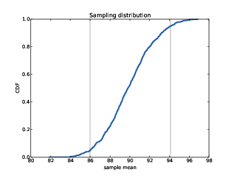
Figure 8.1: Sampling distribution of x, with confidence interval.
In each iteration, we choose n values from a normal
distribution with the given parameters, and compute the sample mean,
xbar. We run 1000 simulations and then compute the
distribution, cdf, of the estimates. The result is shown in
Figure 8.1. This distribution is called the sampling distribution of the estimator. It shows how much the
estimates would vary if we ran the experiment over and over.
The mean of the sampling distribution is pretty close to the hypothetical value of µ, which means that the experiment yields the right answer, on average. After 1000 tries, the lowest result is 82 kg, and the highest is 98 kg. This range suggests that the estimate might be off by as much as 8 kg.
There are two common ways to summarize the sampling distribution:
- Standard error (SE) is a measure of how far we expect the estimate to be off, on average. For each simulated experiment, we compute the error, x − µ, and then compute the root mean squared error (RMSE). In this example, it is roughly 2.5 kg.
- A confidence interval (CI) is a range that includes a given fraction of the sampling distribution. For example, the 90% confidence interval is the range from the 5th to the 95th percentile. In this example, the 90% CI is (86, 94) kg.
Standard errors and confidence intervals are the source of much confusion:
- People often confuse standard error and standard deviation.
Remember that standard deviation describes variability in a measured
quantity; in this example, the standard deviation of gorilla weight
is 7.5 kg. Standard error describes variability in an estimate. In
this example, the standard error of the mean, based on a sample of 9
measurements, is 2.5 kg.
One way to remember the difference is that, as sample size increases, standard error gets smaller; standard deviation does not.
- People often think that there is a 90% probability that the
actual parameter, µ, falls in the 90% confidence interval.
Sadly, that is not true. If you want to make a claim like that, you
have to use Bayesian methods (see my book, Think Bayes).
The sampling distribution answers a different question: it gives you a sense of how reliable an estimate is by telling you how much it would vary if you ran the experiment again.
It is important to remember that confidence intervals and standard errors only quantify sampling error; that is, error due to measuring only part of the population. The sampling distribution does not account for other sources of error, notably sampling bias and measurement error, which are the topics of the next section.
8.4 Sampling bias
Suppose that instead of the weight of gorillas in a nature preserve, you want to know the average weight of women in the city where you live. It is unlikely that you would be allowed to choose a representative sample of women and weigh them.
A simple alternative would be “telephone sampling;” that is, you could choose random numbers from the phone book, call and ask to speak to an adult woman, and ask how much she weighs.
Telephone sampling has obvious limitations. For example, the sample is limited to people whose telephone numbers are listed, so it eliminates people without phones (who might be poorer than average) and people with unlisted numbers (who might be richer). Also, if you call home telephones during the day, you are less likely to sample people with jobs. And if you only sample the person who answers the phone, you are less likely to sample people who share a phone line.
If factors like income, employment, and household size are related to weight—and it is plausible that they are—the results of your survey would be affected one way or another. This problem is called sampling bias because it is a property of the sampling process.
This sampling process is also vulnerable to self-selection, which is a kind of sampling bias. Some people will refuse to answer the question, and if the tendency to refuse is related to weight, that would affect the results.
Finally, if you ask people how much they weigh, rather than weighing them, the results might not be accurate. Even helpful respondents might round up or down if they are uncomfortable with their actual weight. And not all respondents are helpful. These inaccuracies are examples of measurement error.
When you report an estimated quantity, it is useful to report standard error, or a confidence interval, or both, in order to quantify sampling error. But it is also important to remember that sampling error is only one source of error, and often it is not the biggest.
8.5 Exponential distributions
Let’s play one more round of the estimation game. I’m thinking of a distribution. It’s an exponential distribution, and here’s a sample:
[5.384, 4.493, 19.198, 2.790, 6.122, 12.844]
What do you think is the parameter, λ, of this distribution?
In general, the mean of an exponential distribution is 1/λ, so working backwards, we might choose
| L = 1 / x |
L is an estimator of λ. And not just any estimator; it is also the maximum likelihood estimator (see http://wikipedia.org/wiki/Exponential_distribution#Maximum_likelihood). So if you want to maximize your chance of guessing λ exactly, L is the way to go.
But we know that x is not robust in the presence of outliers, so we expect L to have the same problem.
We can choose an alternative based on the sample median. The median of an exponential distribution is ln(2) / λ, so working backwards again, we can define an estimator
| Lm = ln(2) / m |
To test the performance of these estimators, we can simulate the sampling process:
def Estimate3(n=7, m=1000):
    lam = 2

    means = []
    medians = []
    for _ in range(m):
        xs = np.random.exponential(1.0/lam, n)
        L = 1 / np.mean(xs)
        Lm = math.log(2) / thinkstats2.Median(xs)
        means.append(L)
        medians.append(Lm)

    print('rmse L', RMSE(means, lam))
    print('rmse Lm', RMSE(medians, lam))
    print('mean error L', MeanError(means, lam))
    print('mean error Lm', MeanError(medians, lam))
When I run this experiment with λ=2, the RMSE of L is 1.1. For the median-based estimator Lm, RMSE is 1.8. We can’t tell from this experiment whether L minimizes MSE, but at least it seems better than Lm.
Sadly, it seems that both estimators are biased. For L the mean
error is 0.33; for Lm it is 0.45. And neither converges to 0
as m increases.
It turns out that x is an unbiased estimator of the mean of the distribution, 1 / λ, but L is not an unbiased estimator of λ.
8.6 Exercises
For the following exercises, you can find starter code in
chap08ex.ipynb. Solutions are in chap08soln.py
In this chapter we used x and median to estimate µ, and found that x yields lower MSE. Also, we used S2 and Sn−12 to estimate σ, and found that S2 is biased and Sn−12 unbiased.
Run similar experiments to see if x and median are biased estimates of µ. Also check whether S2 or Sn−12 yields a lower MSE.
Suppose you draw a sample with size n=10 from an exponential distribution with λ=2. Simulate this experiment 1000 times and plot the sampling distribution of the estimate L. Compute the standard error of the estimate and the 90% confidence interval.
Repeat the experiment with a few different values of n and make a plot of standard error versus n.
In games like hockey and soccer, the time between goals is roughly exponential. So you could estimate a team’s goal-scoring rate by observing the number of goals they score in a game. This estimation process is a little different from sampling the time between goals, so let’s see how it works.
Write a function that takes a goal-scoring rate, lam, in goals
per game, and simulates a game by generating the time between goals
until the total time exceeds 1 game, then returns the number of goals
scored.
Write another function that simulates many games, stores the
estimates of lam, then computes their mean error and RMSE.
Is this way of making an estimate biased? Plot the sampling
distribution of the estimates and the 90% confidence interval. What
is the standard error? What happens to sampling error for increasing
values of lam?
8.7 Glossary
- estimation: The process of inferring the parameters of a distribution from a sample.
- estimator: A statistic used to estimate a parameter.
- mean squared error (MSE): A measure of estimation error.
- root mean squared error (RMSE): The square root of MSE, a more meaningful representation of typical error magnitude.
- maximum likelihood estimator (MLE): An estimator that computes the point estimate most likely to be correct.
- bias (of an estimator): The tendency of an estimator to be above or below the actual value of the parameter, when averaged over repeated experiments.
- sampling error: Error in an estimate due to the limited size of the sample and variation due to chance.
- sampling bias: Error in an estimate due to a sampling process that is not representative of the population.
- measurement error: Error in an estimate due to inaccuracy collecting or recording data.
- sampling distribution: The distribution of a statistic if an experiment is repeated many times.
- standard error: The RMSE of an estimate, which quantifies variability due to sampling error (but not other sources of error).
- confidence interval: An interval that represents the expected range of an estimator if an experiment is repeated many times.


