|
This HTML version of is provided for convenience, but it is not the best format for the book. In particular, some of the symbols are not rendered correctly. You might prefer to read the PDF version, or you can buy a hardcopy here. Chapter 6 Operations on distributions6.1 SkewnessSkewness is a statistic that measures the asymmetry of a distribution. Given a sequence of values, xi, the sample skewness is:
You might recognize m2 as the mean squared deviation (also known as variance); m3 is the mean cubed deviation. Negative skewness indicates that a distribution “skews left;” that is, it extends farther to the left than the right. Positive skewness indicates that a distribution skews right. In practice, computing the skewness of a sample is usually not a good idea. If there are any outliers, they have a disproportionate effect on g1. Another way to evaluate the asymmetry of a distribution is to look at the relationship between the mean and median. Extreme values have more effect on the mean than the median, so in a distribution that skews left, the mean is less than the median. Pearson’s median skewness coefficient is an alternative measure of skewness that explicitly captures the relationship between the mean, µ, and the median, µ1/2:
This statistic is robust, which means that it is less vulnerable to the effect of outliers. Exercise 1
Write a function named Skewness that computes
g1 for a sample. Compute the skewness for the distributions of pregnancy length and birth weight. Are the results consistent with the shape of the distributions? Write a function named PearsonSkewness that computes gp for these distributions. How does gp compare to g1? Exercise 2
The “Lake Wobegon effect” is an amusing nickname1 for illusory superiority, which is the tendency for people to
overestimate their abilities relative to others. For example, in some
surveys, more than 80% of respondents believe that they are better
than the average driver (see
http://wikipedia.org/wiki/Illusory_superiority).
If we interpret “average” to mean median, then this result is logically impossible, but if “average” is the mean, this result is possible, although unlikely. What percentage of the population has more than the average number of legs? Exercise 3
The Internal Revenue Service of the United States (IRS) provides data
about income taxes, and other statistics, at http://irs.gov/taxstats.
If you did Exercise 4.13, you have already worked with this data;
otherwise, follow the instructions there to extract the distribution
of incomes from this dataset.
What fraction of the population reports a taxable income below the mean? Compute the median, mean, skewness and Pearson’s skewness of the income data. Because the data has been binned, you will have to make some approximations. The Gini coefficient is a measure of income inequality. Read about it at http://wikipedia.org/wiki/Gini_coefficient and write a function called Gini that computes it for the income distribution. Hint: use the PMF to compute the relative mean difference (see http://wikipedia.org/wiki/Mean_difference). You can download a solution to this exercise from http://thinkstats.com/gini.py. 6.2 Random VariablesA random variable represents a process that generates a random number. Random variables are usually written with a capital letter, like X. When you see a random variable, you should think “a value selected from a distribution.” For example, the formal definition of the cumulative distribution function is: CDFX(x) = P(X ≤ x) I have avoided this notation until now because it is so awful, but here’s what it means: The CDF of the random variable X, evaluated for a particular value x, is defined as the probability that a value generated by the random process X is less than or equal to x. As a computer scientist, I find it helpful to think of a random variable as an object that provides a method, which I will call generate, that uses a random process to generate values. For example, here is a definition for a class that represents random variables: class RandomVariable(object):
"""Parent class for all random variables."""
And here is a random variable with an exponential distribution: class Exponential(RandomVariable):
def __init__(self, lam):
self.lam = lam
def generate(self):
return random.expovariate(self.lam)
The init method takes the parameter, λ, and stores it as an attribute. The generate method returns a random value from the exponential distribution with that parameter. Each time you invoke generate, you get a different value. The value you get is called a random variate, which is why many function names in the random module include the word “variate.” If I were just generating exponential variates, I would not bother to define a new class; I would use random.expovariate. But for other distributions it might be useful to use RandomVariable objects. For example, the Erlang distribution is a continuous distribution with parameters λ and k (see http://wikipedia.org/wiki/Erlang_distribution). One way to generate values from an Erlang distribution is to add k values from an exponential distribution with the same λ. Here’s an implementation: class Erlang(RandomVariable):
def __init__(self, lam, k):
self.lam = lam
self.k = k
self.expo = Exponential(lam)
def generate(self):
total = 0
for i in range(self.k):
total += self.expo.generate()
return total
The init method creates an Exponential object with the given parameter; then generate uses it. In general, the init method can take any set of parameters and the generate function can implement any random process. Exercise 4
Write a definition for a class that represents a random variable
with a Gumbel distribution (see http://wikipedia.org/wiki/Gumbel_distribution).
6.3 PDFsThe derivative of a CDF is called a probability density function, or PDF. For example, the PDF of an exponential distribution is
The PDF of a normal distribution is
Evaluating a PDF for a particular value of x is usually not useful. The result is not a probability; it is a probability density. In physics, density is mass per unit of volume; in order to get a mass, you have to multiply by volume or, if the density is not constant, you have to integrate over volume. Similarly, probability density measures probability per unit of x. In order to get a probability mass2, you have to integrate over x. For example, if x is a random variable whose PDF is PDFX, we can compute the probability that a value from X falls between −0.5 and 0.5:
Or, since the CDF is the integral of the PDF, we can write
For some distributions we can evaluate the CDF explicitly, so we would use the second option. Otherwise we usually have to integrate the PDF numerically. Exercise 5
What is the probability that a value chosen from an exponential distribution with parameter λ falls between 1 and 20? Express your answer as a function of λ. Keep this result handy; we will use it in Section 8.8. Exercise 6
In the BRFSS (see Section 4.5), the distribution of
heights is roughly normal with parameters µ = 178 cm and
σ2 = 59.4 cm for men, and µ = 163 cm and σ2 = 52.8 cm for
women.
In order to join Blue Man Group, you have to be male between 5’10” and 6’1” (see http://bluemancasting.com). What percentage of the U.S. male population is in this range? Hint: see Section 4.3. 6.4 ConvolutionSuppose we have two random variables, X and Y, with distributions CDFX and CDFY. What is the distribution of the sum Z = X + Y? One option is to write a RandomVariable object that generates the sum: class Sum(RandomVariable):
def __init__(X, Y):
self.X = X
self.Y = Y
def generate():
return X.generate() + Y.generate()
Given any RandomVariables, X and Y, we can create a Sum object that represents Z. Then we can use a sample from Zto approximate CDFZ. This approach is simple and versatile, but not very efficient; we have to generate a large sample to estimate CDFZ accurately, and even then it is not exact. If CDFX and CDFY are expressed as functions, sometimes we can find CDFZ exactly. Here’s how:
As an example, suppose X and Y are random variables with an exponential distribution with parameter λ. The distribution of Z = X + Yis:
Now we have to remember that PDFexpo is 0 for all negative values, but we can handle that by adjusting the limits of integration:
Now we can combine terms and move constants outside the integral:
This, it turns out, is the PDF of an Erlang distribution with parameter k = 2 (see http://wikipedia.org/wiki/Erlang_distribution). So the convolution of two exponential distributions (with the same parameter) is an Erlang distribution. Exercise 7
If X has an exponential distribution with parameter
λ, and Y has an Erlang distribution with parameters
k and λ, what is the distribution of the sum Z = X + Y?
Exercise 8
Suppose I draw two values from a distribution; what is the distribution
of the larger value? Express your answer in terms of the PDF or CDF of
the distribution.
As the number of values increases, the distribution of the maximum converges on one of the extreme value distributions; see http://wikipedia.org/wiki/Gumbel_distribution. Exercise 9
If you are given Pmf objects, you can compute the distribution of
the sum by enumerating all pairs of values:
for x in pmf_x.Values():
    for y in pmf_y.Values():
        z = x + y
Write a function that takes PMFX and PMFY and returns a new Pmf that represents the distribution of the sum Z = X + Y. Write a similar function that computes the PMF of Z = max(X, Y). 6.5 Why normal?I said earlier that normal distributions are amenable to analysis, but I didn’t say why. One reason is that they are closed under linear transformation and convolution. To explain what that means, it will help to introduce some notation. If the distribution of a random variable, X, is normal with parameters µ and σ, you can write X ∼ N(µ, σ) where the symbol ∼ means “is distributed” and the script letter N stands for “normal.” A linear transformation of X is something like X’ = aX + b, where aand b are real numbers. A family of distributions is closed under linear transformation if X’ is in the same family as X. The normal distribution has this property; if X ∼ N(µ, σ2), X’ ∼ N(aµ + b, a2 σ) Normal distributions are also closed under convolution. If Z = X + Yand X ∼ N(µX, σX2) and Y ∼ N(µY, σY2) then
The other distributions we have looked at do not have these properties. Exercise 10
If
X ∼ N(µX, σX2) and
Y ∼ N(µY, σY2), what
is the distribution of Z = aX + bY? Exercise 11
Let’s see what happens when we add values from
other distributions. Choose a pair of distributions (any two of
exponential, normal, lognormal, and Pareto) and choose parameters
that make their mean and variance similar.
Generate random numbers from these distributions and compute the distribution of their sums. Use the tests from Chapter 4 to see if the sum can be modeled by a continuous distribution. 6.6 Central limit theoremSo far we have seen:
But it turns out that if we add up a large number of values from almost any distribution, the distribution of the sum converges to normal. More specifically, if the distribution of the values has mean and standard deviation µ and σ, the distribution of the sum is approximately N(nµ, nσ2). This is called the Central Limit Theorem. It is one of the most useful tools for statistical analysis, but it comes with caveats:
The Central Limit Theorem explains, at least in part, the prevalence of normal distributions in the natural world. Most characteristics of animals and other life forms are affected by a large number of genetic and environmental factors whose effect is additive. The characteristics we measure are the sum of a large number of small effects, so their distribution tends to be normal. Exercise 12
If I draw a sample, x1 .. xn, independently from a
distribution with finite mean µ and variance σ2, what is
the distribution of the sample mean:
Exercise 13
Choose a distribution (one of exponential, lognormal or Pareto) and
choose values for the parameter(s). Generate samples with sizes
2, 4, 8, etc., and compute the distribution of their sums. Use
a normal probability plot to see if the distribution is approximately
normal. How many terms do you have to add to see convergence?
Exercise 14
Instead of the distribution of sums, compute the distribution of
products; what happens as the number of terms increases?
Hint: look at the distribution of the log of the products.
6.7 The distribution framework
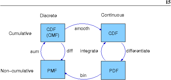
At this point we have seen PMFs, CDFs and PDFs; let’s take a minute to review. Figure 6.1 shows how these functions relate to each other. We started with PMFs, which represent the probabilities for a discrete set of values. To get from a PMF to a CDF, we computed a cumulative sum. To be more consistent, a discrete CDF should be called a cumulative mass function (CMF), but as far as I can tell no one uses that term. To get from a CDF to a PMF, you can compute differences in cumulative probabilities. Similarly, a PDF is the derivative of a continuous CDF; or, equivalently, a CDF is the integral of a PDF. But remember that a PDF maps from values to probability densities; to get a probability, you have to integrate. To get from a discrete to a continuous distribution, you can perform various kinds of smoothing. One form of smoothing is to assume that the data come from an analytic continuous distribution (like exponential or normal) and to estimate the parameters of that distribution. And that’s what Chapter 8 is about. If you divide a PDF into a set of bins, you can generate a PMF that is at least an approximation of the PDF. We use this technique in Chapter 8 to do Bayesian estimation. Exercise 15
Write a function called MakePmfFromCdf that takes a Cdf object
and returns the corresponding Pmf object. You can find a solution to this exercise in thinkstats.com/Pmf.py. 6.8 Glossary
|
Like this book?
Are you using one of our books in a class?We'd like to know about it. Please consider filling out this short survey.
|