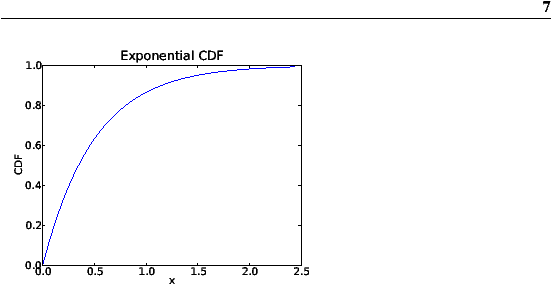
This HTML version of is provided for convenience, but it is not the best format for the book. In particular, some of the symbols are not rendered correctly.

You might prefer to read the PDF version, or you can buy a hardcopy here.

Chapter 4  Continuous distributions

The distributions we have used so far are called empirical distributions because they are based on empirical observations, which are necessarily finite samples.

The alternative is a continuous distribution, which is characterized by a CDF that is a continuous function (as opposed to a step function). Many real world phenomena can be approximated by continuous distributions.

4.1  The exponential distribution

I’ll start with the exponential distribution because it is easy to work with. In the real world, exponential distributions come up when we look at a series of events and measure the times between events, which are called interarrival times. If the events are equally likely to occur at any time, the distribution of interarrival times tends to look like an exponential distribution.

The CDF of the exponential distribution is:

The parameter, λ, determines the shape of the distribution. Figure 4.1 shows what this CDF looks like with λ = 2.

---

Figure 4.1: CDF of exponential distribution.

---

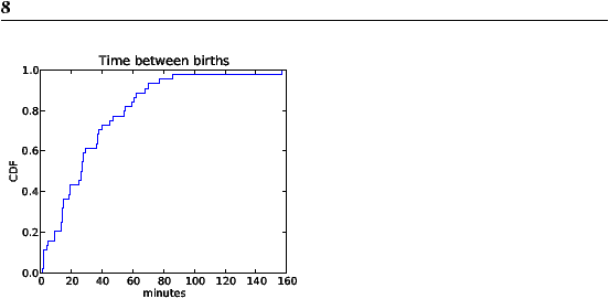
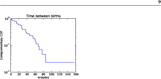
In general, the mean of an exponential distribution is 1/λ, so the mean of this distribution is 0.5. The median is log(2)/λ, which is roughly 0.35.

To see an example of a distribution that is approximately exponential, we will look at the interarrival time of babies. On December 18, 1997, 44 babies were born in a hospital in Brisbane, Australia¹. The times of birth for all 44 babies were reported in the local paper; you can download the data from http://thinkstats.com/babyboom.dat.

Figure 4.2 shows the CDF of the interarrival times in minutes. It seems to have the general shape of an exponential distribution, but how can we tell?

One way is to plot the complementary CDF, 1 − CDF(x), on a log-y scale. For data from an exponential distribution, the result is a straight line. Let’s see why that works.

If you plot the complementary CDF (CCDF) of a dataset that you think is exponential, you expect to see a function like:

Taking the log of both sides yields:

   log y ≈ -λx

So on a log-y scale the CCDF is a straight line with slope −λ.

---

Figure 4.2: CDF of interarrival times

---

---

Figure 4.3: CCDF of interarrival times.

---

Figure 4.3 shows the CCDF of the interarrivals on a log-y scale. It is not exactly straight, which suggests that the exponential distribution is only an approximation. Most likely the underlying assumption—that a birth is equally likely at any time of day—is not exactly true.

myplot.Cdf(cdf, complement=True, xscale='linear', yscale='log') 

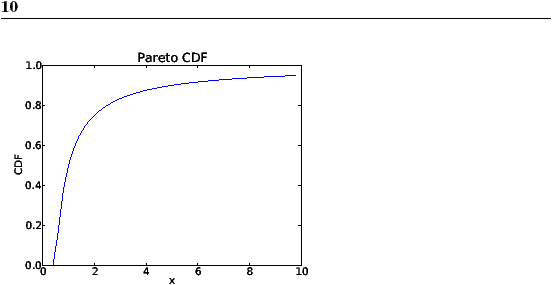
4.2  The Pareto distribution

The Pareto distribution is named after the economist Vilfredo Pareto, who used it to describe the distribution of wealth (see http://wikipedia.org/wiki/Pareto_distribution). Since then, it has been used to describe phenomena in the natural and social sciences including sizes of cities and towns, sand particles and meteorites, forest fires and earthquakes.

The CDF of the Pareto distribution is:

The parameters x_m and α determine the location and shape of the distribution. x_m is the minimum possible value. Figure 4.4 shows the CDF of a Pareto distribution with parameters x_m = 0.5 and α = 1.

---

Figure 4.4: CDF of a Pareto distribution.

---

The median of this distribution is x_m 2^1/α, which is 1, but the 95th percentile is 10. By contrast, the exponential distribution with median 1 has 95th percentile of only 1.5.

There is a simple visual test that indicates whether an empirical distribution fits a Pareto distribution: on a log-log scale, the CCDF looks like a straight line. If you plot a the CCDF of a sample from a Pareto distribution on a linear scale, you expect to see a function like:

Taking the log of both sides yields:

   log y ≈−α (log x − log x_m)

So if you plot log y versus log x, it should look like a straight line with slope −α and intercept −α log x_m.

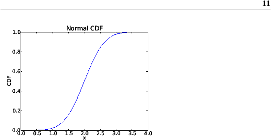
4.3  The normal distribution

The normal distribution, also called Gaussian, is the most commonly used because it describes so many phenomena, at least approximately. It turns out that there is a good reason for its ubiquity, which we will get to in Section 6.6.

The normal distribution has many properties that make it amenable for analysis, but the CDF is not one of them. Unlike the other distributions we have looked at, there is no closed-form expression for the normal CDF; the most common alternative is to write it in terms of the error function, which is a special function written erf(x):

The parameters µ and σ determine the mean and standard deviation of the distribution.

If these formulas make your eyes hurt, don’t worry; they are easy to implement in Python². There are many fast and accurate ways to approximate erf(x). You can download one of them from http://thinkstats.com/erf.py, which provides functions named erf and NormalCdf.

Figure 4.5 shows the CDF of the normal distribution with parameters µ = 2.0 and σ = 0.5. The sigmoid shape of this curve is a recognizable characteristic of a normal distribution.

---

Figure 4.5: CDF of a normal distribution.

---

In the previous chapter we looked at the distribution of birth weights in the NSFG. Figure 4.6 shows the empirical CDF of weights for all live births and the CDF of a normal distribution with the same mean and variance.

---

Figure 4.6: CDF of birth weights with a normal model.

---

The normal distribution is a good model for this dataset. A model is a useful simplification. In this case it is useful because we can summarize the entire distribution with just two numbers, µ = 116.5 and σ = 19.9, and the resulting error (difference between the model and the data) is small.

Below the 10th percentile there is a discrepancy between the data and the model; there are more light babies than we would expect in a normal distribution. If we are interested in studying preterm babies, it would be important to get this part of the distribution right, so it might not be appropriate to use the normal model.

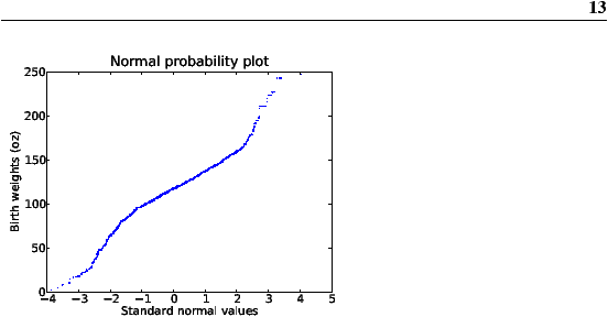
4.4  Normal probability plot

For the exponential, Pareto and Weibull distributions, there are simple transformations we can use to test whether a continuous distribution is a good model of a dataset.

For the normal distribution there is no such transformation, but there is an alternative called a normal probability plot. It is based on rankits: if you generate n values from a normal distribution and sort them, the kth rankit is the mean of the distribution for the kth value.

Computing rankits exactly is moderately difficult, but there are numerical methods for approximating them. And there is a quick-and-dirty method that is even easier to implement:

1. From a normal distribution with µ = 0 and σ = 1, generate a sample with the same size as your dataset and sort it.
2. Sort the values in the dataset.
3. Plot the sorted values from your dataset versus the random values.

For large datasets, this method works well. For smaller datasets, you can improve it by generating m(n+1) − 1 values from a normal distribution, where n is the size of the dataset and m is a multiplier. Then select every mth element, starting with the mth.

This method works with other distributions as well, as long as you know how to generate a random sample.

Figure 4.7 is a quick-and-dirty normal probability plot for the birth weight data.

---

Figure 4.7: Normal probability plot of birth weights.

---

The curvature in this plot suggests that there are deviations from a normal distribution; nevertheless, it is a good (enough) model for many purposes.

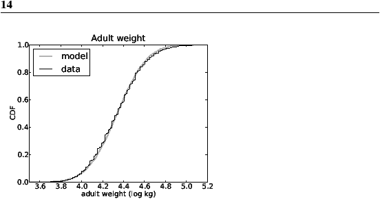
4.5  The lognormal distribution

If the logarithms of a set of values have a normal distribution, the values have a lognormal distribution. The CDF of the lognormal distribution is the same as the CDF of the normal distribution, with log xsubstituted for x.

   CDF_lognormal(x) = CDF_normal(log x)

The parameters of the lognormal distribution are usually denoted µ and σ. But remember that these parameters are not the mean and standard deviation; the mean of a lognormal distribution is exp(µ + σ²/2) and the standard deviation is ugly⁵.

It turns out that the distribution of weights for adults is approximately lognormal⁶.

The National Center for Chronic Disease Prevention and Health Promotion conducts an annual survey as part of the Behavioral Risk Factor Surveillance System (BRFSS)⁷. In 2008, they interviewed 414,509 respondents and asked about their demographics, health and health risks.

---

Figure 4.8: CDF of adult weights (log transform).

---

Among the data they collected are the weights in kilograms of 398,484 respondents. Figure 4.8 shows the distribution of log w, where wis weight in kilograms, along with a normal model.

The normal model is a good fit for the data, although the highest weights exceed what we expect from the normal model even after the log transform. Since the distribution of log wfits a normal distribution, we conclude that wfits a lognormal distribution.

4.6  Why model?

At the beginning of this chapter I said that many real world phenomena can be modeled with continuous distributions. “So,” you might ask, “what?”

Like all models, continuous distributions are abstractions, which means they leave out details that are considered irrelevant. For example, an observed distribution might have measurement errors or quirks that are specific to the sample; continuous models smooth out these idiosyncrasies.

Continuous models are also a form of data compression. When a model fits a dataset well, a small set of parameters can summarize a large amount of data.

It is sometimes surprising when data from a natural phenomenon fit a continuous distribution, but these observations can lead to insight into physical systems. Sometimes we can explain why an observed distribution has a particular form. For example, Pareto distributions are often the result of generative processes with positive feedback (so-called preferential attachment processes: see http://wikipedia.org/wiki/Preferential_attachment.).

Continuous distributions lend themselves to mathematical analysis, as we will see in Chapter 6.

4.7  Generating random numbers

Continuous CDFs are also useful for generating random numbers. If there is an efficient way to compute the inverse CDF, ICDF(p), we can generate random values with the appropriate distribution by choosing from a uniform distribution from 0 to 1, then choosing

   x = ICDF(p)

For example, the CDF of the exponential distribution is

Solving for x yields:

   x= −log (1 − p) / λ

So in Python we can write

def expovariate(lam):
    p = random.random()
    x = -math.log(1-p) / lam
    return x

I called the parameter lam because lambda is a Python keyword. Most implementations of random.random can return 0 but not 1, so 1 − p can be 1 but not 0, which is good, because log 0 is undefined.

4.8  Glossary

empirical distribution:

The distribution of values in a sample.

continuous distribution:

A distribution described by a continuous function.

interarrival time:

The elapsed time between two events.

error function:

A special mathematical function, so-named because it comes up in the study of measurement errors.

normal probability plot:

A plot of the sorted values in a sample versus the expected value for each if their distribution is normal.

rankit:

The expected value of an element in a sorted list of values from a normal distribution.

model:

A useful simplification. Continuous distributions are often good models of more complex empirical distributions.

corpus:

A body of text used as a sample of a language.

hapaxlegomenon:

A word that appears only once in a corpus. It appears twice in this book, so far.

1

This example is based on information and data from Dunn, “A Simple Dataset for Demonstrating Common Distributions,” Journal of Statistics Education v.7, n.3 (1999).

2

As of Python 3.2, it is even easier; erf is in the math module.

3

Whether it does or not is a fascinating controversy that I invite you to investigate at your leisure.

4

On this topic, you might be interested to read http://wikipedia.org/wiki/Christopher_Langan.

5

See http://wikipedia.org/wiki/Log-normal_distribution.

6

I was tipped off to this possibility by a comment (without citation) at http://mathworld.wolfram.com/LogNormalDistribution.html. Subsequently I found a paper that proposes the log transform and suggests a cause: Penman and Johnson, “The Changing Shape of the Body Mass Index Distribution Curve in the Population,” Preventing Chronic Disease, 2006 July; 3(3): A74. Online at http://www.ncbi.nlm.nih.gov/pmc/articles/PMC1636707.

7

Centers for Disease Control and Prevention (CDC). Behavioral Risk Factor Surveillance System Survey Data. Atlanta, Georgia: U.S. Department of Health and Human Services, Centers for Disease Control and Prevention, 2008.

Like this book?

Are you using one of our books in a class?