This HTML version of Think Bayes is provided for convenience, but it is not the best format for the book. In particular, some of the math symbols are not rendered correctly.

You might prefer to read the PDF version, or you can buy a hard copy from Amazon.

Chapter 15 Dealing with Dimensions

15.1 Belly button bacteria

Belly Button Biodiversity 2.0 (BBB2) is a nation-wide citizen science project with the goal of identifying bacterial species that can be found in human navels (http://bbdata.yourwildlife.org). The project might seem whimsical, but it is part of an increasing interest in the human microbiome, the set of microorganisms that live on human skin and parts of the body.

In their pilot study, BBB2 researchers collected swabs from the navels of 60 volunteers, used multiplex pyrosequencing to extract and sequence fragments of 16S rDNA, then identified the species or genus the fragments came from. Each identified fragment is called a “read.”

We can use these data to answer several related questions:

Based on the number of species observed, can we estimate the total number of species in the environment?
Can we estimate the prevalence of each species; that is, the fraction of the total population belonging to each species?
If we are planning to collect additional samples, can we predict how many new species we are likely to discover?
How many additional reads are needed to increase the fraction of observed species to a given threshold?

These questions make up what is called the Unseen Species problem.

15.2 Lions and tigers and bears

I’ll start with a simplified version of the problem where we know that there are exactly three species. Let’s call them lions, tigers and bears. Suppose we visit a wild animal preserve and see 3 lions, 2 tigers and one bear.

If we have an equal chance of observing any animal in the preserve, the number of each species we see is governed by the multinomial distribution. If the prevalence of lions and tigers and bears is p_lion and p_tiger and p_bear, the likelihood of seeing 3 lions, 2 tigers and one bear is proportional to

p_lion**3 * p_tiger**2 * p_bear**1

An approach that is tempting, but not correct, is to use beta distributions, as in Section 4.5, to describe the prevalence of each species separately. For example, we saw 3 lions and 3 non-lions; if we think of that as 3 “heads” and 3 “tails,” then the posterior distribution of p_lion is:

    beta = thinkbayes.Beta()
    beta.Update((3, 3))
    print beta.MaximumLikelihood()

The maximum likelihood estimate for p_lion is the observed rate, 50%. Similarly the MLEs for p_tiger and p_bear are 33% and 17%.

But there are two problems:

We have implicitly used a prior for each species that is uniform from 0 to 1, but since we know that there are three species, that prior is not correct. The right prior should have a mean of 1/3, and there should be zero likelihood that any species has a prevalence of 100%.
The distributions for each species are not independent, because the prevalences have to add up to 1. To capture this dependence, we need a joint distribution for the three prevalences.

We can use a Dirichlet distribution to solve both of these problems (see http://en.wikipedia.org/wiki/Dirichlet_distribution). In the same way we used the beta distribution to describe the distribution of bias for a coin, we can use a Dirichlet distribution to describe the joint distribution of p_lion, p_tiger and p_bear.

The Dirichlet distribution is the multi-dimensional generalization of the beta distribution. Instead of two possible outcomes, like heads and tails, the Dirichlet distribution handles any number of outcomes: in this example, three species.

If there are n outcomes, the Dirichlet distribution is described by n parameters, written α₁ through α_n.

Here’s the definition, from thinkbayes.py, of a class that represents a Dirichlet distribution:

class Dirichlet(object):

    def __init__(self, n):
        self.n = n
        self.params = numpy.ones(n, dtype=numpy.int)

n is the number of dimensions; initially the parameters are all 1. I use a numpy array to store the parameters so I can take advantage of array operations.

Given a Dirichlet distribution, the marginal distribution for each prevalence is a beta distribution, which we can compute like this:

    def MarginalBeta(self, i):
        alpha0 = self.params.sum()
        alpha = self.params[i]
        return Beta(alpha, alpha0-alpha)

i is the index of the marginal distribution we want. alpha0 is the sum of the parameters; alpha is the parameter for the given species.

In the example, the prior marginal distribution for each species is Beta(1, 2). We can compute the prior means like this:

    dirichlet = thinkbayes.Dirichlet(3)
    for i in range(3):
        beta = dirichlet.MarginalBeta(i)
        print beta.Mean()

As expected, the prior mean prevalence for each species is 1/3.

To update the Dirichlet distribution, we add the observations to the parameters like this:

    def Update(self, data):
        m = len(data)
        self.params[:m] += data

Here data is a sequence of counts in the same order as params, so in this example, it should be the number of lions, tigers and bears.

data can be shorter than params; in that case there are some species that have not been observed.

Here’s code that updates dirichlet with the observed data and computes the posterior marginal distributions.

    data = [3, 2, 1]
    dirichlet.Update(data)

    for i in range(3):
        beta = dirichlet.MarginalBeta(i)
        pmf = beta.MakePmf()
        print i, pmf.Mean()

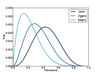
Figure 15.1: Distribution of prevalences for three species.

Figure 15.1 shows the results. The posterior mean prevalences are 44%, 33%, and 22%.

15.3 The hierarchical version

We have solved a simplified version of the problem: if we know how many species there are, we can estimate the prevalence of each.

Now let’s get back to the original problem, estimating the total number of species. To solve this problem I’ll define a meta-Suite, which is a Suite that contains other Suites as hypotheses. In this case, the top-level Suite contains hypotheses about the number of species; the bottom level contains hypotheses about prevalences.

Here’s the class definition:

class Species(thinkbayes.Suite):

    def __init__(self, ns):
        hypos = [thinkbayes.Dirichlet(n) for n in ns]
        thinkbayes.Suite.__init__(self, hypos)

__init__ takes a list of possible values for n and makes a list of Dirichlet objects.

Here’s the code that creates the top-level suite:

    ns = range(3, 30)
    suite = Species(ns)

ns is the list of possible values for n. We have seen 3 species, so there have to be at least that many. I chose an upper bound that seems reasonable, but we will check later that the probability of exceeding this bound is low. And at least initially we assume that any value in this range is equally likely.

To update a hierarchical model, you have to update all levels. Usually you have to update the bottom level first and work up, but in this case we can update the top level first:

#class Species

    def Update(self, data):
        thinkbayes.Suite.Update(self, data)
        for hypo in self.Values():
            hypo.Update(data)

Species.Update invokes Update in the parent class, then loops through the sub-hypotheses and updates them.

Now all we need is a likelihood function:

# class Species

    def Likelihood(self, data, hypo):
        dirichlet = hypo
        like = 0
        for i in range(1000):
            like += dirichlet.Likelihood(data)

        return like

data is a sequence of observed counts; hypo is a Dirichlet object. Species.Likelihood calls Dirichlet.Likelihood 1000 times and returns the total.

Why call it 1000 times? Because Dirichlet.Likelihood doesn’t actually compute the likelihood of the data under the whole Dirichlet distribution. Instead, it draws one sample from the hypothetical distribution and computes the likelihood of the data under the sampled set of prevalences.

Here’s what it looks like:

# class Dirichlet

    def Likelihood(self, data):
        m = len(data)
        if self.n < m:
            return 0

        x = data
        p = self.Random()
        q = p[:m]**x
        return q.prod()

The length of data is the number of species observed. If we see more species than we thought existed, the likelihood is 0.

Otherwise we select a random set of prevalences, p, and compute the multinomial PMF, which is

c_x p₁^x₁ ⋯ p_n^x_n

p_i is the prevalence of the ith species, and x_i is the observed number. The first term, c_x, is the multinomial coefficient; I leave it out of the computation because it is a multiplicative factor that depends only on the data, not the hypothesis, so it gets normalized away (see http://en.wikipedia.org/wiki/Multinomial_distribution).

m is the number of observed species. We only need the first m elements of p; for the others, x_i is 0, so p_i^x_i is 1, and we can leave them out of the product.

15.4 Random sampling

There are two ways to generate a random sample from a Dirichlet distribution. One is to use the marginal beta distributions, but in that case you have to select one at a time and scale the rest so they add up to 1 (see http://en.wikipedia.org/wiki/Dirichlet_distribution#Random_number_generation).

A less obvious, but faster, way is to select values from n gamma distributions, then normalize by dividing through by the total. Here’s the code:

# class Dirichlet

    def Random(self):
        p = numpy.random.gamma(self.params)
        return p / p.sum()

Now we’re ready to look at some results. Here is the code that extracts the posterior distribution of n:

    def DistOfN(self):
        pmf = thinkbayes.Pmf()
        for hypo, prob in self.Items():
            pmf.Set(hypo.n, prob)
        return pmf

DistOfN iterates through the top-level hypotheses and accumulates the probability of each n.

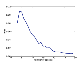
Figure 15.2: Posterior distribution of n.

Figure 15.2 shows the result. The most likely value is 4. Values from 3 to 7 are reasonably likely; after that the probabilities drop off quickly. The probability that there are 29 species is low enough to be negligible; if we chose a higher bound, we would get nearly the same result.

Remember that this result is based on a uniform prior for n. If we have background information about the number of species in the environment, we might choose a different prior.

15.5 Optimization

I have to admit that I am proud of this example. The Unseen Species problem is not easy, and I think this solution is simple and clear, and takes surprisingly few lines of code (about 50 so far).

The only problem is that it is slow. It’s good enough for the example with only 3 observed species, but not good enough for the belly button data, with more than 100 species in some samples.

The next few sections present a series of optimizations we need to make this solution scale. Before we get into the details, here’s a road map.

The first step is to recognize that if we update the Dirichlet distributions with the same data, the first m parameters are the same for all of them. The only difference is the number of hypothetical unseen species. So we don’t really need n Dirichlet objects; we can store the parameters in the top level of the hierarchy. Species2 implements this optimization.
Species2 also uses the same set of random values for all of the hypotheses. This saves time generating random values, but it has a second benefit that turns out to be more important: by giving all hypotheses the same selection from the sample space, we make the comparison between the hypotheses more fair, so it takes fewer iterations to converge.
Even with these changes there is a major performance problem. As the number of observed species increases, the array of random prevalences gets bigger, and the chance of choosing one that is approximately right becomes small. So the vast majority of iterations yield small likelihoods that don’t contribute much to the total, and don’t discriminate between hypotheses.
The solution is to do the updates one species at a time. Species4 is a simple implementation of this strategy using Dirichlet objects to represent the sub-hypotheses.
Finally, Species5 combines the sub-hypotheses into the top level and uses numpy array operations to speed things up.

If you are not interested in the details, feel free to skip to Section 15.9 where we look at results from the belly button data.

15.6 Collapsing the hierarchy

All of the bottom-level Dirichlet distributions are updated with the same data, so the first m parameters are the same for all of them. We can eliminate them and merge the parameters into the top-level suite. Species2 implements this optimization:

class Species2(object):
    
    def __init__(self, ns):
        self.ns = ns
        self.probs = numpy.ones(len(ns), dtype=numpy.double)
        self.params = numpy.ones(self.high, dtype=numpy.int)

ns is the list of hypothetical values for n; probs is the list of corresponding probabilities. And params is the sequence of Dirichlet parameters, initially all 1.

Species2.Update updates both levels of the hierarchy: first the probability for each value of n, then the Dirichlet parameters:

# class Species2

    def Update(self, data):
        like = numpy.zeros(len(self.ns), dtype=numpy.double)
        for i in range(1000):
            like += self.SampleLikelihood(data)

        self.probs *= like
        self.probs /= self.probs.sum()

        m = len(data)
        self.params[:m] += data

SampleLikelihood returns an array of likelihoods, one for each value of n. like accumulates the total likelihood for 1000 samples. self.probs is multiplied by the total likelihood, then normalized. The last two lines, which update the parameters, are the same as in Dirichlet.Update.

Now let’s look at SampleLikelihood. There are two opportunities for optimization here:

When the hypothetical number of species, n, exceeds the observed number, m, we only need the first m terms of the multinomial PMF; the rest are 1.
If the number of species is large, the likelihood of the data might be too small for floating-point (see 10.5). So it is safer to compute log-likelihoods.

Again, the multinomial PMF is

c_x p₁^x₁ ⋯ p_n^x_n

So the log-likelihood is

logc_x + x₁ logp₁ + ⋯ + x_n logp_n

which is fast and easy to compute. Again, c_x it is the same for all hypotheses, so we can drop it. Here’s the code:

# class Species2

    def SampleLikelihood(self, data):
        gammas = numpy.random.gamma(self.params)

        m = len(data)
        row = gammas[:m]
        col = numpy.cumsum(gammas)

        log_likes = []
        for n in self.ns:
            ps = row / col[n-1]
            terms = data * numpy.log(ps)
            log_like = terms.sum()
            log_likes.append(log_like)

        log_likes -= numpy.max(log_likes)
        likes = numpy.exp(log_likes)

        coefs = [thinkbayes.BinomialCoef(n, m) for n in self.ns]
        likes *= coefs

        return likes

gammas is an array of values from a gamma distribution; its length is the largest hypothetical value of n. row is just the first m elements of gammas; since these are the only elements that depend on the data, they are the only ones we need.

For each value of n we need to divide row by the total of the first n values from gamma. cumsum computes these cumulative sums and stores them in col.

The loop iterates through the values of n and accumulates a list of log-likelihoods.

Inside the loop, ps contains the row of probabilities, normalized with the appropriate cumulative sum. terms contains the terms of the summation, x_i logp_i, and log_like contains their sum.

After the loop, we want to convert the log-likelihoods to linear likelihoods, but first it’s a good idea to shift them so the largest log-likelihood is 0; that way the linear likelihoods are not too small (see 10.5).

Finally, before we return the likelihood, we have to apply a correction factor, which is the number of ways we could have observed these m species, if the total number of species is n. BinomialCoefficient computes “n choose m”, which is written (

As often happens, the optimized version is less readable and more error-prone than the original. But that’s one reason I think it is a good idea to start with the simple version; we can use it for regression testing. I plotted results from both versions and confirmed that they are approximately equal, and that they converge as the number of iterations increases.

15.7 One more problem

There’s more we could do to optimize this code, but there’s another problem we need to fix first. As the number of observed species increases, this version gets noisier and takes more iterations to converge on a good answer.

The problem is that if the prevalences we choose from the Dirichlet distribution, the ps, are not at least approximately right, the likelihood of the observed data is close to zero and almost equally bad for all values of n. So most iterations don’t provide any useful contribution to the total likelihood. And as the number of observed species, m, gets large, the probability of choosing ps with non-negligible likelihood gets small. Really small.

Fortunately, there is a solution. Remember that if you observe a set of data, you can update the prior distribution with the entire dataset, or you can break it up into a series of updates with subsets of the data, and the result is the same either way.

For this example, the key is to perform the updates one species at a time. That way when we generate a random set of ps, only one of them affects the computed likelihood, so the chance of choosing a good one is much better.

Here’s a new version that updates one species at a time:

class Species4(Species):

    def Update(self, data):
        m = len(data)

        for i in range(m):
            one = numpy.zeros(i+1)
            one[i] = data[i]            
            Species.Update(self, one)

This version inherits __init__ from Species, so it represents the hypotheses as a list of Dirichlet objects (unlike Species2).

Update loops through the observed species and makes an array, one, with all zeros and one species count. Then it calls Update in the parent class, which computes the likelihoods and updates the sub-hypotheses.

So in the running example, we do three updates. The first is something like “I have seen three lions.” The second is “I have seen two tigers and no additional lions.” And the third is “I have seen one bear and no more lions and tigers.”

Here’s the new version of Likelihood:

# class Species4

    def Likelihood(self, data, hypo):
        dirichlet = hypo
        like = 0
        for i in range(self.iterations):
            like += dirichlet.Likelihood(data)

        # correct for the number of unseen species the new one
        # could have been
        m = len(data)
        num_unseen = dirichlet.n - m + 1
        like *= num_unseen

        return like

This is almost the same as Species.Likelihood. The difference is the factor, num_unseen. This correction is necessary because each time we see a species for the first time, we have to consider that there were some number of other unseen species that we might have seen. For larger values of n there are more unseen species that we could have seen, which increases the likelihood of the data.

This is a subtle point and I have to admit that I did not get it right the first time. But again I was able to validate this version by comparing it to the previous versions.

15.8 We’re not done yet

Performing the updates one species at a time solves one problem, but it creates another. Each update takes time proportional to k m, where k is the number of hypotheses and m is the number of observed species. So if we do m updates, the total run time is proportional to k m².

But we can speed things up using the same trick we used in Section 15.6: we’ll get rid of the Dirichlet objects and collapse the two levels of the hierarchy into a single object. So here’s yet another version of Species:

class Species5(Species2):
    
    def Update(self, data):
        m = len(data)
        for i in range(m):
            self.UpdateOne(i+1, data[i])
            self.params[i] += data[i]

This version inherits __init__ from Species2, so it uses ns and probs to represent the distribution of n, and params to represent the parameters of the Dirichlet distribution.

Update is similar to what we saw in the previous section. It loops through the observed species and calls UpdateOne:

# class Species5

    def UpdateOne(self, i, count):
        likes = numpy.zeros(len(self.ns), dtype=numpy.double)
        for i in range(self.iterations):
            likes += self.SampleLikelihood(i, count)

        unseen_species = [n-i+1 for n in self.ns]
        likes *= unseen_species

        self.probs *= likes
        self.probs /= self.probs.sum()

This function is similar to Species2.Update, with two changes:

The interface is different. Instead of the whole dataset, we get i, the index of the observed species, and count, how many of that species we’ve seen.
We have to apply a correction factor for the number of unseen species, as in Species4.Likelihood. The difference here is that we update all of the likelihoods at once with array multiplication.

Finally, here’s SampleLikelihood:

# class Species5

    def SampleLikelihood(self, i, count):
        gammas = numpy.random.gamma(self.params)

        sums = numpy.cumsum(gammas)[self.ns[0]-1:]

        ps = gammas[i-1] / sums
        log_likes = numpy.log(ps) * count

        log_likes -= numpy.max(log_likes)
        likes = numpy.exp(log_likes)

        return likes

This is similar to Species2.SampleLikelihood; the difference is that each update only includes a single species, so we don’t need a loop.

The runtime of this function is proportional to the number of hypotheses, k. It runs m times, so the run time of the update is proportional to k m. And the number of iterations we need to get an accurate result is usually small.

15.9 The belly button data

That’s enough about lions and tigers and bears. Let’s get back to belly buttons. To get a sense of what the data look like, consider subject B1242, whose sample of 400 reads yielded 61 species with the following counts:

92, 53, 47, 38, 15, 14, 12, 10, 8, 7, 7, 5, 5, 
4, 4, 4, 4, 4, 4, 4, 3, 3, 3, 3, 3, 3, 3, 2, 2, 2, 2,
1, 1, 1, 1, 1, 1, 1, 1, 1, 1, 1, 1, 1, 1, 1, 1, 1, 1,
1, 1, 1, 1, 1, 1, 1, 1, 1, 1, 1, 1

There are a few dominant species that make up a large fraction of the whole, but many species that yielded only a single read. The number of these “singletons” suggests that there are likely to be at least a few unseen species.

In the example with lions and tigers, we assume that each animal in the preserve is equally likely to be observed. Similarly, for the belly button data, we assume that each bacterium is equally likely to yield a read.

In reality, each step in the data-collection process might introduce biases. Some species might be more likely to be picked up by a swab, or to yield identifiable amplicons. So when we talk about the prevalence of each species, we should remember this source of error.

I should also acknowledge that I am using the term “species” loosely. First, bacterial species are not well defined. Second, some reads identify a particular species, others only identify a genus. To be more precise, I should say “operational taxonomic unit”, or OTU.

Now let’s process some of the belly button data. I define a class called Subject to represent information about each subject in the study:

class Subject(object):

    def __init__(self, code):
        self.code = code
        self.species = []

Each subject has a string code, like “B1242”, and a list of (count, species name) pairs, sorted in increasing order by count. Subject provides several methods to make it easy to access these counts and species names. You can see the details in http://thinkbayes.com/species.py. For more information see Section 0.3.

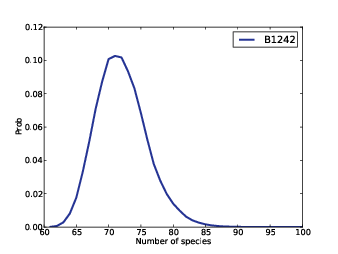
Figure 15.3: Distribution of n for subject B1242.

Subject provides a method named Process that creates and updates a Species5 suite, which represents the distributions of n and the prevalences.

And Suite2 provides DistOfN, which returns the posterior distribution of n.

# class Suite2

    def DistN(self):
        items = zip(self.ns, self.probs)
        pmf = thinkbayes.MakePmfFromItems(items)
        return pmf

Figure 15.3 shows the distribution of n for subject B1242. The probability that there are exactly 61 species, and no unseen species, is nearly zero. The most likely value is 72, with 90% credible interval 66 to 79. At the high end, it is unlikely that there are as many as 87 species.

Next we compute the posterior distribution of prevalence for each species. Species2 provides DistOfPrevalence:

# class Species2

    def DistOfPrevalence(self, index):
        metapmf = thinkbayes.Pmf()

        for n, prob in zip(self.ns, self.probs):
            beta = self.MarginalBeta(n, index)
            pmf = beta.MakePmf()
            metapmf.Set(pmf, prob)

        mix = thinkbayes.MakeMixture(metapmf)
        return metapmf, mix

index indicates which species we want. For each n, we have a different posterior distribution of prevalence.

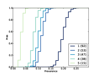
Figure 15.4: Distribution of prevalences for subject B1242.

The loop iterates through the possible values of n and their probabilities. For each value of n it gets a Beta object representing the marginal distribution for the indicated species. Remember that Beta objects contain the parameters alpha and beta; they don’t have values and probabilities like a Pmf, but they provide MakePmf, which generates a discrete approximation to the continuous beta distribution.

metapmf is a meta-Pmf that contains the distributions of prevalence, conditioned on n. MakeMixture combines the meta-Pmf into mix, which combines the conditional distributions into a single distribution of prevalence.

Figure 15.4 shows results for the five species with the most reads. The most prevalent species accounts for 23% of the 400 reads, but since there are almost certainly unseen species, the most likely estimate for its prevalence is 20%, with 90% credible interval between 17% and 23%.

15.10 Predictive distributions

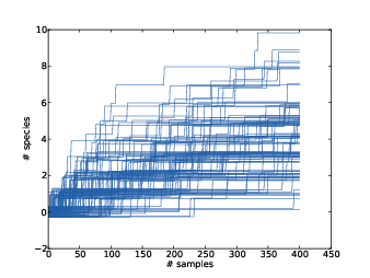
Figure 15.5: Simulated rarefaction curves for subject B1242.

I introduced the hidden species problem in the form of four related questions. We have answered the first two by computing the posterior distribution for n and the prevalence of each species.

The other two questions are:

If we are planning to collect additional reads, can we predict how many new species we are likely to discover?
How many additional reads are needed to increase the fraction of observed species to a given threshold?

To answer predictive questions like this we can use the posterior distributions to simulate possible future events and compute predictive distributions for the number of species, and fraction of the total, we are likely to see.

The kernel of these simulations looks like this:

Choose n from its posterior distribution.
Choose a prevalence for each species, including possible unseen species, using the Dirichlet distribution.
Generate a random sequence of future observations.
Compute the number of new species, num_new, as a function of the number of additional reads, k.
Repeat the previous steps and accumulate the joint distribution of num_new and k.

And here’s the code. RunSimulation runs a single simulation:

# class Subject

    def RunSimulation(self, num_reads):
        m, seen = self.GetSeenSpecies()
        n, observations = self.GenerateObservations(num_reads)

        curve = []
        for k, obs in enumerate(observations):
            seen.add(obs)

            num_new = len(seen) - m
            curve.append((k+1, num_new))

        return curve

num_reads is the number of additional reads to simulate. m is the number of seen species, and seen is a set of strings with a unique name for each species. n is a random value from the posterior distribution, and observations is a random sequence of species names.

Each time through the loop, we add the new observation to seen and record the number of reads and the number of new species so far.

The result of RunSimulation is a rarefaction curve, represented as a list of pairs with the number of reads and the number of new species.

Before we see the results, let’s look at GetSeenSpecies and GenerateObservations.

#class Subject

    def GetSeenSpecies(self):
        names = self.GetNames()
        m = len(names)
        seen = set(SpeciesGenerator(names, m))
        return m, seen

GetNames returns the list of species names that appear in the data files, but for many subjects these names are not unique. So I use SpeciesGenerator to extend each name with a serial number:

def SpeciesGenerator(names, num):
    i = 0
    for name in names:
        yield '%s-%d' % (name, i)
        i += 1

    while i < num:
        yield 'unseen-%d' % i
        i += 1

Given a name like Corynebacterium, SpeciesGenerator yields Corynebacterium-1. When the list of names is exhausted, it yields names like unseen-62.

Here is GenerateObservations:

# class Subject

    def GenerateObservations(self, num_reads):
        n, prevalences = self.suite.SamplePosterior()

        names = self.GetNames()
        name_iter = SpeciesGenerator(names, n)

        d = dict(zip(name_iter, prevalences))
        cdf = thinkbayes.MakeCdfFromDict(d)
        observations = cdf.Sample(num_reads)

        return n, observations

Again, num_reads is the number of additional reads to generate. n and prevalences are samples from the posterior distribution.

cdf is a Cdf object that maps species names, including the unseen, to cumulative probabilities. Using a Cdf makes it efficient to generate a random sequence of species names.

Finally, here is Species2.SamplePosterior:

    def SamplePosterior(self):
        pmf = self.DistOfN()
        n = pmf.Random()
        prevalences = self.SamplePrevalences(n)
        return n, prevalences

And SamplePrevalences, which generates a sample of prevalences conditioned on n:

# class Species2

    def SamplePrevalences(self, n):
        params = self.params[:n]
        gammas = numpy.random.gamma(params)
        gammas /= gammas.sum()
        return gammas

We saw this algorithm for generating random values from a Dirichlet distribution in Section 15.4.

Figure 15.5 shows 100 simulated rarefaction curves for subject B1242. The curves are “jittered;” that is, I shifted each curve by a random offset so they would not all overlap. By inspection we can estimate that after 400 more reads we are likely to find 2–6 new species.

15.11 Joint posterior

Figure 15.6: Distributions of the number of new species conditioned on the number of additional reads.

We can use these simulations to estimate the joint distribution of num_new and k, and from that we can get the distribution of num_new conditioned on any value of k.

def MakeJointPredictive(curves):
    joint = thinkbayes.Joint()
    for curve in curves:
        for k, num_new in curve:
            joint.Incr((k, num_new))
    joint.Normalize()
    return joint

MakeJointPredictive makes a Joint object, which is a Pmf whose values are tuples.

curves is a list of rarefaction curves created by RunSimulation. Each curve contains a list of pairs of k and num_new.

The resulting joint distribution is a map from each pair to its probability of occurring. Given the joint distribution, we can use Joint.Conditional get the distribution of num_new conditioned on k (see Section 9.6).

Subject.MakeConditionals takes a list of ks and computes the conditional distribution of num_new for each k. The result is a list of Cdf objects.

def MakeConditionals(curves, ks):
    joint = MakeJointPredictive(curves)

    cdfs = []
    for k in ks:
        pmf = joint.Conditional(1, 0, k)
        pmf.name = 'k=%d' % k
        cdf = pmf.MakeCdf()
        cdfs.append(cdf)

    return cdfs

Figure 15.6 shows the results. After 100 reads, the median predicted number of new species is 2; the 90% credible interval is 0 to 5. After 800 reads, we expect to see 3 to 12 new species.

15.12 Coverage

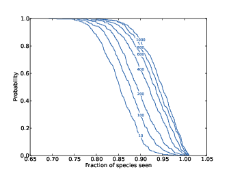
Figure 15.7: Complementary CDF of coverage for a range of additional reads.

The last question we want to answer is, “How many additional reads are needed to increase the fraction of observed species to a given threshold?”

To answer this question, we need a version of RunSimulation that computes the fraction of observed species rather than the number of new species.

# class Subject

    def RunSimulation(self, num_reads):
        m, seen = self.GetSeenSpecies()
        n, observations = self.GenerateObservations(num_reads)

        curve = []
        for k, obs in enumerate(observations):
            seen.add(obs)

            frac_seen = len(seen) / float(n)
            curve.append((k+1, frac_seen))

        return curve

Next we loop through each curve and make a dictionary, d, that maps from the number of additional reads, k, to a list of fracs; that is, a list of values for the coverage achieved after k reads.

    def MakeFracCdfs(self, curves):
        d = {}
        for curve in curves:
            for k, frac in curve:
                d.setdefault(k, []).append(frac)

        cdfs = {}
        for k, fracs in d.iteritems():
            cdf = thinkbayes.MakeCdfFromList(fracs)
            cdfs[k] = cdf

        return cdfs

Then for each value of k we make a Cdf of fracs; this Cdf represents the distribution of coverage after k reads.

Remember that the CDF tells you the probability of falling below a given threshold, so the complementary CDF tells you the probability of exceeding it. Figure 15.7 shows complementary CDFs for a range of values of k.

To read this figure, select the level of coverage you want to achieve along the x-axis. As an example, choose 90%.

Now you can read up the chart to find the probability of achieving 90% coverage after k reads. For example, with 200 reads, you have about a 40% chance of getting 90% coverage. With 1000 reads, you have a 90% chance of getting 90% coverage.

With that, we have answered the four questions that make up the unseen species problem. To validate the algorithms in this chapter with real data, I had to deal with a few more details. But this chapter is already too long, so I won’t discuss them here.

You can read about the problems, and how I addressed them, at http://allendowney.blogspot.com/2013/05/belly-button-biodiversity-end-game.html.

You can download the code in this chapter from http://thinkbayes.com/species.py. For more information see Section 0.3.

15.13 Discussion

The Unseen Species problem is an area of active research, and I believe the algorithm in this chapter is a novel contribution. So in fewer than 200 pages we have made it from the basics of probability to the research frontier. I’m very happy about that.

My goal for this book is to present three related ideas:

Bayesian thinking: The foundation of Bayesian analysis is the idea of using probability distributions to represent uncertain beliefs, using data to update those distributions, and using the results to make predictions and inform decisions.
A computational approach: The premise of this book is that it is easier to understand Bayesian analysis using computation rather than math, and easier to implement Bayesian methods with reusable building blocks that can be rearranged to solve real-world problems quickly.
Iterative modeling: Most real-world problems involve modeling decisions and trade-offs between realism and complexity. It is often impossible to know ahead of time what factors should be included in the model and which can be abstracted away. The best approach is to iterate, starting with simple models and adding complexity gradually, using each model to validate the others.

These ideas are versatile and powerful; they are applicable to problems in every area of science and engineering, from simple examples to topics of current research.

If you made it this far, you should be prepared to apply these tools to new problems relevant to your work. I hope you find them useful; let me know how it goes!