This HTML version of Think Complexity, 2nd Edition is provided for convenience, but it is not the best format of the book. In particular, some of the symbols are not rendered correctly.

You might prefer to read the PDF version.

Chapter 3  Small World Graphs

Many networks in the real world, including social networks, have the “small world property”, which is that the average distance between nodes, measured in number of edges on the shortest path, is much smaller than expected.

In this chapter, I present Stanley Milgram’s famous Small World Experiment, which was the first demonstration of the small world property in a real social network. Then we’ll consider Watts-Strogatz graphs, which are intended as a model of small world graphs. I’ll replicate the experiment Watts and Strogatz performed and explain what it is intended to show.

Along the way, we’ll see two new graph algorithms: breadth-first search (BFS) and Dijkstra’s algorithm for computing the shortest path between nodes in a graph.

The code for this chapter is in chap03.ipynb in the repository for this book. More information about working with the code is in Section ??.

3.1  Stanley Milgram

Stanley Milgram was an American social psychologist who conducted two of the most famous experiments in social science, the Milgram experiment, which studied people’s obedience to authority (http://thinkcomplex.com/milgram) and the Small World Experiment, which studied the structure of social networks (http://thinkcomplex.com/small).

In the Small World Experiment, Milgram sent a package to several randomly-chosen people in Wichita, Kansas, with instructions asking them to forward an enclosed letter to a target person, identified by name and occupation, in Sharon, Massachusetts (which happens to be the town near Boston where I grew up). The subjects were told that they could mail the letter directly to the target person only if they knew him personally; otherwise they were instructed to send it, and the same instructions, to a relative or friend they thought would be more likely to know the target person.

Many of the letters were never delivered, but for the ones that were the average path length — the number of times the letters were forwarded — was about six. This result was taken to confirm previous observations (and speculations) that the typical distance between any two people in a social network is about “six degrees of separation”.

This conclusion is surprising because most people expect social networks to be localized — people tend to live near their friends — and in a graph with local connections, path lengths tend to increase in proportion to geographical distance. For example, most of my friends live nearby, so I would guess that the average distance between nodes in a social network is about 50 miles. Wichita is about 1600 miles from Boston, so if Milgram’s letters traversed typical links in the social network, they should have taken 32 hops, not 6.

3.2  Watts and Strogatz

In 1998 Duncan Watts and Steven Strogatz published a paper in Nature, “Collective dynamics of ‘small-world’ networks”, that proposed an explanation for the small world phenomenon. You can download it from http://thinkcomplex.com/watts.

Watts and Strogatz start with two kinds of graph that were well understood: random graphs and regular graphs. In a random graph, nodes are connected at random. In a regular graph, every node has the same number of neighbors. They consider two properties of these graphs, clustering and path length:

• Clustering is a measure of the “cliquishness” of the graph. In a graph, a clique is a subset of nodes that are all connected to each other; in a social network, a clique is a set of people who are all friends with each other. Watts and Strogatz defined a clustering coefficient that quantifies the likelihood that two nodes that are connected to the same node are also connected to each other.

• Path length is a measure of the average distance between two nodes, which corresponds to the degrees of separation in a social network.

Watts and Strogatz show that regular graphs have high clustering and high path lengths, whereas random graphs with the same size usually have low clustering and low path lengths. So neither of these is a good model of social networks, which combine high clustering with short path lengths.

Their goal was to create a generative model of a social network. A generative model tries to explain a phenomenon by modeling the process that builds or leads to the phenomenon. Watts and Strogatz proposed this process for building small-world graphs:

1. Start with a regular graph with n nodes and each node connected to k neighbors.
2. Choose a subset of the edges and “rewire” them by replacing them with random edges.

The probability that an edge is rewired is a parameter, p, that controls how random the graph is. With p=0, the graph is regular; with p=1 it is completely random.

Watts and Strogatz found that small values of p yield graphs with high clustering, like a regular graph, and low path lengths, like a random graph.

In this chapter I replicate the Watts and Strogatz experiment in the following steps:

1. We’ll start by constructing a ring lattice, which is a kind of regular graph.
2. Then we’ll rewire it as Watts and Strogatz did.
3. We’ll write a function to measure the degree of clustering and use a NetworkX function to compute path lengths.
4. Then we’ll compute the degree of clustering and path length for a range of values of p.
5. Finally, I’ll present Dijkstra’s algorithm, which computes shortest paths efficiently.

3.3  Ring lattice

---

Figure 3.1: A ring lattice with n=10 and k=4.

---

A regular graph is a graph where each node has the same number of neighbors; the number of neighbors is also called the degree of the node.

A ring lattice is a kind of regular graph, which Watts and Strogatz use as the basis of their model. In a ring lattice with n nodes, the nodes can be arranged in a circle with each node connected to the k nearest neighbors.

For example, a ring lattice with n=3 and k=2 would contain the following edges: (0, 1), (1, 2), and (2, 0). Notice that the edges “wrap around” from the highest-numbered node back to 0.

More generally, we can enumerate the edges like this:

adjacent_edges takes a list of nodes and a parameter, halfk, which is half of k. It is a generator function that yields one edge at a time. It uses the modulus operator, %, to wrap around from the highest-numbered node to the lowest.

We can test it like this:

Now we can use adjacent_edges to make a ring lattice:

Notice that make_ring_lattice uses floor division to compute halfk, so it is only correct if k is even. If k is odd, floor division rounds down, so the result is a ring lattice with degree k-1. As one of the exercises at the end of the chapter, you will generate regular graphs with odd values of k.

We can test make_ring_lattice like this:

Figure ?? shows the result.

3.4  WS graphs

---

Figure 3.2: WS graphs with n=20, k=4, and p=0 (left), p=0.2 (middle), and p=1 (right).

---

To make a Watts-Strogatz (WS) graph, we start with a ring lattice and “rewire” some of the edges. In their paper, Watts and Strogatz consider the edges in a particular order and rewire each one with probability p. If an edge is rewired, they leave the first node unchanged and choose the second node at random. They don’t allow self loops or multiple edges; that is, you can’t have a edge from a node to itself, and you can’t have more than one edge between the same two nodes.

Here is my implementation of this process.

The parameter p is the probability of rewiring an edge. The for loop enumerates the edges and uses flip (defined in Section ??) to choose which ones get rewired.

If we are rewiring an edge from node u to node v, we have to choose a replacement for v, called new_v.

1. To compute the possible choices, we start with nodes, which is a set, and subtract off u and its neighbors, which avoids self loops and multiple edges.
2. To choose new_v, we use the NumPy function choice, which is in the module random.

3. Then we remove the existing edge from u to v, and
4. Add a new edge from u to new_v.

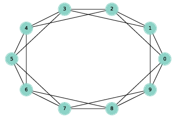
As an aside, the expression G[u] returns a dictionary that contains the neighbors of u as keys. It is usually faster than using G.neighbors (see http://thinkcomplex.com/neigh).

This function does not consider the edges in the order specified by Watts and Strogatz, but that doesn’t seem to affect the results.

Figure ?? shows WS graphs with n=20, k=4, and a range of values of p. When p=0, the graph is a ring lattice. When p=1, it is completely random. As we’ll see, the interesting things happen in between.

3.5  Clustering

The next step is to compute the clustering coefficient, which quantifies the tendency for the nodes to form cliques. A clique is a set of nodes that are completely connected; that is, there are edges between all pairs of nodes in the set.

Suppose a particular node, u, has k neighbors. If all of the neighbors are connected to each other, there would be k(k−1)/2 edges among them. The fraction of those edges that actually exist is the local clustering coefficient for u, denoted C_u.

If we compute the average of C_u over all nodes, we get the “network average clustering coefficient”, denoted C.

Here is a function that computes it.

Again I use G[u], which returns a dictionary with the neighbors of u as keys.

If a node has fewer than 2 neighbors, the clustering coefficient is undefined, so we return np.nan, which is a special value that indicates “Not a Number”.

Otherwise we compute the number of possible edges among the neighbors, count the number of those edges that actually exist, and return the fraction that exist.

We can test the function like this:

In a ring lattice with k=4, the clustering coefficient for each node is 0.5 (if you are not convinced, take another look at Figure ??).

Now we can compute the network average clustering coefficient like this:

The NumPy function nanmean computes the mean of the local clustering coefficients, ignoring any values that are NaN.

We can test clustering_coefficient like this:

In this graph, the local clustering coefficient for all nodes is 0.5, so the average across nodes is 0.5. Of course, we expect this value to be different for WS graphs.

3.6  Shortest path lengths

The next step is to compute the characteristic path length, L, which is the average length of the shortest path between each pair of nodes. To compute it, I’ll start with a function provided by NetworkX, shortest_path_length. I’ll use it to replicate the Watts and Strogatz experiment, then I’ll explain how it works.

Here’s a function that takes a graph and returns a list of shortest path lengths, one for each pair of nodes.

The return value from nx.shortest_path_length is a dictionary of dictionaries. The outer dictionary maps from each node, u, to a dictionary that maps from each node, v, to the length of the shortest path from u to v.

With the list of lengths from path_lengths, we can compute L like this:

And we can test it with a small ring lattice:

In this example, all 3 nodes are connected to each other, so the mean path length is 1.

3.7  The WS experiment

---

Figure 3.3: Clustering coefficient (C) and characteristic path length (L) for WS graphs with n=1000, k=10, and a range of p.

---

Now we are ready to replicate the WS experiment, which shows that for a range of values of p, a WS graph has high clustering like a regular graph and short path lengths like a random graph.

I’ll start with run_one_graph, which takes n, k, and p; it generates a WS graph with the given parameters and computes the mean path length, mpl, and clustering coefficient, cc:

Watts and Strogatz ran their experiment with n=1000 and k=10. With these parameters, run_one_graph takes a few seconds on my computer; most of that time is spent computing the mean path length.

Now we need to compute these values for a range of p. I’ll use the NumPy function logspace again to compute ps:

Here’s the function that runs the experiment:

For each value of p, we generate 20 random graphs and average the results. Since the return value from run_one_graph is a pair, t is a list of pairs. When we convert it to an array, we get one row for each iteration and columns for L and C. Calling mean with the option axis=0 computes the mean of each column; the result is an array with one row and two columns.

When the loop exits, means is a list of pairs, which we convert to a NumPy array with one row for each value of p and columns for L and C.

We can extract the columns like this:

In order to plot L and C on the same axes, we standardize them by dividing through by the first element:

Figure ?? shows the results. As p increases, the mean path length drops quickly, because even a small number of randomly rewired edges provide shortcuts between regions of the graph that are far apart in the lattice. On the other hand, removing local links decreases the clustering coefficient much more slowly.

As a result, there is a wide range of p where a WS graph has the properties of a small world graph, high clustering and low path lengths.

And that’s why Watts and Strogatz propose WS graphs as a model for real-world networks that exhibit the small world phenomenon.

3.8  What kind of explanation is that?

If you ask me why planetary orbits are elliptical, I might start by modeling a planet and a star as point masses; I would look up the law of universal gravitation at http://thinkcomplex.com/grav and use it to write a differential equation for the motion of the planet. Then I would either derive the orbit equation or, more likely, look it up at http://thinkcomplex.com/orbit. With a little algebra, I could derive the conditions that yield an elliptical orbit. Then I would argue that the objects we consider planets satisfy these conditions.

People, or at least scientists, are generally satisfied with this kind of explanation. One of the reasons for its appeal is that the assumptions and approximations in the model seem reasonable. Planets and stars are not really point masses, but the distances between them are so big that their actual sizes are negligible. Planets in the same solar system can affect each other’s orbits, but the effect is usually small. And we ignore relativistic effects, again on the assumption that they are small.

This explanation is also appealing because it is equation-based. We can express the orbit equation in a closed form, which means that we can compute orbits efficiently. It also means that we can derive general expressions for the orbital velocity, orbital period, and other quantities.

Finally, I think this kind of explanation is appealing because it has the form of a mathematical proof. It is important to remember that the proof pertains to the model and not the real world. That is, we can prove that an idealized model yields elliptical orbits, but we can’t prove that real orbits are ellipses (in fact, they are not). Nevertheless, the resemblance to a proof is appealing.

By comparison, Watts and Strogatz’s explanation of the small world phenomenon may seem less satisfying. First, the model is more abstract, which is to say less realistic. Second, the results are generated by simulation, not by mathematical analysis. Finally, the results seem less like a proof and more like an example.

Many of the models in this book are like the Watts and Strogatz model: abstract, simulation-based and (at least superficially) less formal than conventional mathematical models. One of the goals of this book is to consider the questions these models raise:

• What kind of work can these models do: are they predictive, or explanatory, or both?
• Are the explanations these models offer less satisfying than explanations based on more traditional models? Why?
• How should we characterize the differences between these and more conventional models? Are they different in kind or only in degree?

Over the course of the book I will offer my answers to these questions, but they are tentative and sometimes speculative. I encourage you to consider them skeptically and reach your own conclusions.

3.9  Breadth-First Search

When we computed shortest paths, we used a function provided by NetworkX, but I have not explained how it works. To do that, I’ll start with breadth-first search, which is the basis of Dijkstra’s algorithm for computing shortest paths.

In Section ?? I presented reachable_nodes, which finds all the nodes that can be reached from a given starting node:

I didn’t say so at the time, but reachable_nodes performs a depth-first search (DFS). Now we’ll modify it to perform breadth-first search (BFS).

To understand the difference, imagine you are exploring a castle. You start in a room with three doors marked A, B, and C. You open door C and discover another room, with doors marked D, E, and F.

Which door do you open next? If you are feeling adventurous, you might want to go deeper into the castle and choose D, E, or F. That would be a depth-first search.

But if you wanted to be more systematic, you might go back and explore A and B before D, E, and F. That would be a breadth-first search.

In reachable_nodes, we use the list method pop to choose the next node to “explore”. By default, pop returns the last element of the list, which is the last one we added. In the example, that would be door F.

If we want to perform a BFS instead, the simplest solution is to pop the first element of the list:

That works, but it is slow. In Python, popping the last element of a list takes constant time, but popping the first element is linear in the length of the list. In the worst case, the length of the stack is O(n), which makes this implementation of BFS O(nm), which is much worse than what it should be, O(n + m).

We can solve this problem with a double-ended queue, also known as a deque. The important feature of a deque is that you can add and remove elements from the beginning or end in constant time. To see how it is implemented, see http://thinkcomplex.com/deque.

Python provides a deque in the collections module, so we can import it like this:

And we can use it to write an efficient BFS:

The differences are:

• I replaced the list called stack with a deque called queue.
• I replaced pop with popleft, which removes and returns the leftmost element of the queue.

This version is back to being O(n + m). Now we’re ready to find shortest paths.

3.10  Dijkstra’s algorithm

Edsger W. Dijkstra was a Dutch computer scientist who invented an efficient shortest-path algorithm (see http://thinkcomplex.com/dijk). He also invented the semaphore, which is a data structure used to coordinate programs that communicate with each other (see http://thinkcomplex.com/sem and Downey, The Little Book of Semaphores).

Dijkstra is famous (and notorious) as the author of a series of essays on computer science. Some, like “A Case against the GO TO Statement”, had a profound effect on programming practice. Others, like “On the Cruelty of Really Teaching Computing Science”, are entertaining in their cantankerousness, but less effective.

Dijkstra’s algorithm solves the “single source shortest path problem”, which means that it finds the minimum distance from a given “source” node to every other node in the graph (or at least every connected node).

I’ll present a simplified version of the algorithm that considers all edges the same length. The more general version works with any non-negative edge lengths.

The simplified version is similar to the breadth-first search in the previous section except that we replace the set called seen with a dictionary called dist, which maps from each node to its distance from the source:

Here’s how it works:

• Initially, queue contains a single element, source, and dist maps from source to distance 0 (which is the distance from source to itself).
• Each time through the loop, we use popleft to select the next node in the queue.
• Next we find all neighbors of node that are not already in dist.
• Since the distance from source to node is dist[node], the distance to any of the undiscovered neighbors is dist[node]+1.
• For each neighbor, we add an entry to dist, then we add the neighbors to the queue.

This algorithm only works if we use BFS, not DFS. To see why, consider this:

1. The first time through the loop node is source, and new_dist is 1. So the neighbors of source get distance 1 and they go in the queue.
2. When we process the neighbors of source, all of their neighbors get distance 2. We know that none of them can have distance 1, because if they did, we would have discovered them during the first iteration.
3. Similarly, when we process the nodes with distance 2, we give their neighbors distance 3. We know that none of them can have distance 1 or 2, because if they did, we would have discovered them during a previous iteration.

And so on. If you are familiar with proof by induction, you can see where this is going.

But this argument only works if we process all nodes with distance 1 before we start processing nodes with distance 2, and so on. And that’s exactly what BFS does.

In the exercises at the end of this chapter, you’ll write a version of Dijkstra’s algorithm using DFS, so you’ll have a chance to see what goes wrong.

3.11  Exercises

Contribute

Pay what you want:

Small $1.00 USD Medium $5.00 USD Large $10.00 USD X-Large $20.00 USD XX-Large $50.00 USD

Are you using one of our books in a class?

Think DSP

Think Java

Think Bayes

Think Python 2e

Think Stats 2e

Think Complexity