Chapter 2  Harmonics

In this chapter I present several new waveforms; we will look at their spectrums to understand their harmonic structure, which is the set of sinusoids they are made up of.

I’ll also introduce one of the most important phenomena in digital signal processing: aliasing. And I’ll explain a little more about how the Spectrum class works.

The code for this chapter is in chap02.ipynb, which is in the repository for this book (see Section 0.2). You can also view it at http://tinyurl.com/thinkdsp02.

2.1  Triangle waves

A sinusoid contains only one frequency component, so its spectrum has only one peak. More complicated waveforms, like the violin recording, yield DFTs with many peaks. In this section we investigate the relationship between waveforms and their spectrums.

---

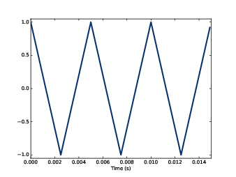
Figure 2.1: Segment of a triangle signal at 200 Hz.

---

I’ll start with a triangle waveform, which is like a straight-line version of a sinusoid. Figure 2.1 shows a triangle waveform with frequency 200 Hz.

To generate a triangle wave, you can use thinkdsp.TriangleSignal:

class TriangleSignal(Sinusoid):

    def evaluate(self, ts):
        cycles = self.freq * ts + self.offset / PI2
        frac, _ = np.modf(cycles)
        ys = np.abs(frac - 0.5)
        ys = normalize(unbias(ys), self.amp)
        return ys

TriangleSignal inherits __init__ from Sinusoid, so it takes the same arguments: freq, amp, and offset.

The only difference is evaluate. As we saw before, ts is the sequence of sample times where we want to evaluate the signal.

There are many ways to generate a triangle wave. The details are not important, but here’s how evaluate works:

1. cycles is the number of cycles since the start time. np.modf splits the number of cycles into the fraction part, stored in frac, and the integer part, which is ignored ¹.
2. frac is a sequence that ramps from 0 to 1 with the given frequency. Subtracting 0.5 yields values between -0.5 and 0.5. Taking the absolute value yields a waveform that zig-zags between 0.5 and 0.
3. unbias shifts the waveform down so it is centered at 0; then normalize scales it to the given amplitude, amp.

Here’s the code that generates Figure 2.1:

signal = thinkdsp.TriangleSignal(200)
signal.plot()

---

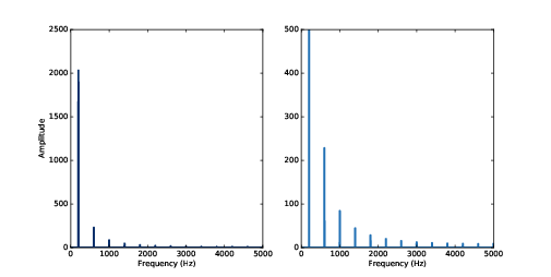
Figure 2.2: Spectrum of a triangle signal at 200 Hz, shown on two vertical scales. The version on the right cuts off the fundamental to show the harmonics more clearly.

---

Next we can use the Signal to make a Wave, and use the Wave to make a Spectrum:

wave = signal.make_wave(duration=0.5, framerate=10000)
spectrum = wave.make_spectrum()
spectrum.plot()

Figure 2.2 shows two views of the result; the view on the right is scaled to show the harmonics more clearly. As expected, the highest peak is at the fundamental frequency, 200 Hz, and there are additional peaks at harmonic frequencies, which are integer multiples of 200.

But one surprise is that there are no peaks at the even multiples: 400, 800, etc. The harmonics of a triangle wave are all odd multiples of the fundamental frequency, in this example 600, 1000, 1400, etc.

Another feature of this spectrum is the relationship between the amplitude and frequency of the harmonics. Their amplitude drops off in proportion to frequency squared. For example the frequency ratio of the first two harmonics (200 and 600 Hz) is 3, and the amplitude ratio is approximately 9. The frequency ratio of the next two harmonics (600 and 1000 Hz) is 1.7, and the amplitude ratio is approximately 1.7² = 2.9. This relationship is called the harmonic structure.

2.2  Square waves

---

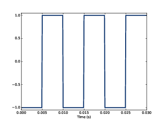
Figure 2.3: Segment of a square signal at 100 Hz.

---

thinkdsp also provides SquareSignal, which represents a square signal. Here’s the class definition:

class SquareSignal(Sinusoid):

    def evaluate(self, ts):
        cycles = self.freq * ts + self.offset / PI2
        frac, _ = np.modf(cycles)
        ys = self.amp * np.sign(unbias(frac))
        return ys

Like TriangleSignal, SquareSignal inherits __init__ from Sinusoid, so it takes the same parameters.

And the evaluate method is similar. Again, cycles is the number of cycles since the start time, and frac is the fractional part, which ramps from 0 to 1 each period.

unbias shifts frac so it ramps from -0.5 to 0.5, then np.sign maps the negative values to -1 and the positive values to 1. Multiplying by amp yields a square wave that jumps between -amp and amp.

---

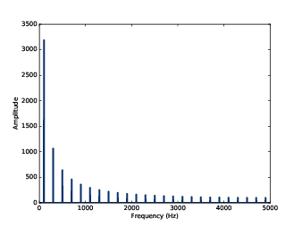
Figure 2.4: Spectrum of a square signal at 100 Hz.

---

Figure 2.3 shows three periods of a square wave with frequency 100 Hz, and Figure 2.4 shows its spectrum.

Like a triangle wave, the square wave contains only odd harmonics, which is why there are peaks at 300, 500, and 700 Hz, etc. But the amplitude of the harmonics drops off more slowly. Specifically, amplitude drops in proportion to frequency (not frequency squared).

The exercises at the end of this chapter give you a chance to explore other waveforms and other harmonic structures.

2.3  Aliasing

---

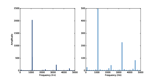
Figure 2.5: Spectrum of a triangle signal at 1100 Hz sampled at 10,000 frames per second. The view on the right is scaled to show the harmonics.

---

I have a confession. I chose the examples in the previous section carefully to avoid showing you something confusing. But now it’s time to get confused.

Figure 2.5 shows the spectrum of a triangle wave at 1100 Hz, sampled at 10,000 frames per second. Again, the view on the right is scaled to show the harmonics.

The harmonics of this wave should be at 3300, 5500, 7700, and 9900 Hz. In the figure, there are peaks at 1100 and 3300 Hz, as expected, but the third peak is at 4500, not 5500 Hz. The fourth peak is at 2300, not 7700 Hz. And if you look closely, the peak that should be at 9900 is actually at 100 Hz. What’s going on?

The problem is that when you evaluate the signal at discrete points in time, you lose information about what happened between samples. For low frequency components, that’s not a problem, because you have lots of samples per period.

But if you sample a signal at 5000 Hz with 10,000 frames per second, you only have two samples per period. That turns out to be enough, just barely, but if the frequency is higher, it’s not.

To see why, let’s generate cosine signals at 4500 and 5500 Hz, and sample them at 10,000 frames per second:

    framerate = 10000

    signal = thinkdsp.CosSignal(4500)
    duration = signal.period*5
    segment = signal.make_wave(duration, framerate=framerate)
    segment.plot()

    signal = thinkdsp.CosSignal(5500)
    segment = signal.make_wave(duration, framerate=framerate)
    segment.plot()

---

Figure 2.6: Cosine signals at 4500 and 5500 Hz, sampled at 10,000 frames per second. The signals are different, but the samples are identical.

---

Figure 2.6 shows the result. I plotted the Signals with thin gray lines and the samples using vertical lines, to make it easier to compare the two Waves. The problem should be clear: even though the Signals are different, the Waves are identical!

When we sample a 5500 Hz signal at 10,000 frames per second, the result is indistinguishable from a 4500 Hz signal. For the same reason, a 7700 Hz signal is indistinguishable from 2300 Hz, and a 9900 Hz is indistinguishable from 100 Hz.

This effect is called aliasing because when the high frequency signal is sampled, it appears to be a low frequency signal.

In this example, the highest frequency we can measure is 5000 Hz, which is half the sampling rate. Frequencies above 5000 Hz are folded back below 5000 Hz, which is why this threshold is sometimes called the “folding frequency”. It is sometimes also called the Nyquist frequency. See http://en.wikipedia.org/wiki/Nyquist_frequency.

The folding pattern continues if the aliased frequency goes below zero. For example, the 5th harmonic of the 1100 Hz triangle wave is at 12,100 Hz. Folded at 5000 Hz, it would appear at -2100 Hz, but it gets folded again at 0 Hz, back to 2100 Hz. In fact, you can see a small peak at 2100 Hz in Figure 2.4, and the next one at 4300 Hz.

2.4  Computing the spectrum

We have seen the Wave method make_spectrum several times. Here is the implementation (leaving out some details we’ll get to later):

from np.fft import rfft, rfftfreq

# class Wave:
    def make_spectrum(self):
        n = len(self.ys)
        d = 1 / self.framerate

        hs = rfft(self.ys)
        fs = rfftfreq(n, d)

        return Spectrum(hs, fs, self.framerate)

The parameter self is a Wave object. n is the number of samples in the wave, and d is the inverse of the frame rate, which is the time between samples.

np.fft is the NumPy module that provides functions related to the Fast Fourier Transform (FFT), which is an efficient algorithm that computes the Discrete Fourier Transform (DFT).

make_spectrum uses rfft, which stands for “real FFT”, because the Wave contains real values, not complex. Later we’ll see the full FFT, which can handle complex signals. The result of rfft, which I call hs, is a NumPy array of complex numbers that represents the amplitude and phase offset of each frequency component in the wave.

The result of rfftfreq, which I call fs, is an array that contains frequencies corresponding to the hs.

To understand the values in hs, consider these two ways to think about complex numbers:

• A complex number is the sum of a real part and an imaginary part, often written x + iy, where i is the imaginary unit, √−1. You can think of x and y as Cartesian coordinates.
• A complex number is also the product of a magnitude and a complex exponential, A e^{i φ}, where A is the magnitude and φ is the angle in radians, also called the “argument”. You can think of A and φ as polar coordinates.

Each value in hs corresponds to a frequency component: its magnitude is proportional to the amplitude of the corresponding component; its angle is the phase offset.

The Spectrum class provides two read-only properties, amps and angles, which return NumPy arrays representing the magnitudes and angles of the hs. When we plot a Spectrum object, we usually plot amps versus fs. Sometimes it is also useful to plot angles versus fs.

Although it might be tempting to look at the real and imaginary parts of hs, you will almost never need to. I encourage you to think of the DFT as a vector of amplitudes and phase offsets that happen to be encoded in the form of complex numbers.

To modify a Spectrum, you can access the hs directly. For example:

spectrum.hs *= 2
spectrum.hs[spectrum.fs > cutoff] = 0

The first line multiples the elements of hs by 2, which doubles the amplitudes of all components. The second line sets to 0 only the elements of hs where the corresponding frequency exceeds some cutoff frequency.

But Spectrum also provides methods to perform these operations:

spectrum.scale(2)
spectrum.low_pass(cutoff)

You can read the documentation of these methods and others at http://greenteapress.com/thinkdsp.html.

At this point you should have a better idea of how the Signal, Wave, and Spectrum classes work, but I have not explained how the Fast Fourier Transform works. That will take a few more chapters.

2.5  Exercises

Solutions to these exercises are in chap02soln.ipynb.

1

Using an underscore as a variable name is a convention that means, “I don’t intend to use this value.”

Are you using one of our books in a class?

Think Bayes

Think Python

Think Stats

Think Complexity