Buy this book at Amazon.com

This HTML version of the book is provided as a convenience, but some math equations are not translated correctly. The PDF version is more reliable.

Chapter 8  Functions of Vectors

8.1  Functions and files

So far we have only put one function in each file. It is also possible to put more than one function in a file, but only the first one, the top-level function can be called from the Command Window. The other helper functions can be called from anywhere inside the file, but not from any other file.

Large programs almost always require more than one function; keeping all the functions in one file is convenient, but it makes debugging difficult because you can’t call helper functions from the Command Window.

To help with this problem, I often use the top-level function to develop and test my helper functions. For example, to write a program for Exercise 2, I would create a file named duck.m and start with a top-level function named duck that takes no input variables and returns no output value.

Then I would write a function named error_func to evaluate the error function for fzero. To test error_func I would call it from duck and then call duck from the Command Window.

Here’s what my first draft might look like:

function res = duck()
    error = error_func(10)
end

function res = error_func(h)
    rho = 0.3;      % density in g / cm^3
    r = 10;         % radius in cm
    res = h;
end

The line res = h isn’t finished yet, but this is enough code to test. Once I finished and tested error_func, I would modify duck to use fzero.

For this problem I might only need two functions, but if there were more, I could write and test them one at a time, and then combine them into a working program.¹

8.2  Physical modeling

Most of the examples so far have been about mathematics; Exercise 2, the “duck problem,” is the first example we have seen of a physical system. If you didn’t work on this exercise, you should at least go back and read it.

This book is supposed to be about physical modeling, so it might be a good idea to explain what that is. Physical modeling is a process for making predictions about physical systems and explaining their behavior. A physical system is something in the real world that we are interested in, like a duck.

The following figure shows the steps of this process: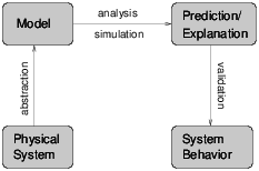

A model is a simplified description of a physical system. The process of building a model is called abstraction. In this context, “abstract” is the opposite of “realistic;” an abstract model bears little direct resemblance to the physical system it models, in the same way that abstract art does not directly depict objects in the real world. A realistic model is one that includes more details and corresponds more directly to the real world.

Abstraction involves making justified decisions about which factors to include in the model and which factors can be simplified or ignored. For example, in the duck problem, we took into account the density of the duck and the buoyancy of water, but we ignored the buoyancy of the duck due to displacement of air and the dynamic effect of paddling feet. We also simplified the geometry of the duck by assuming that the underwater parts of a duck are similar to a segment of a sphere. And we used coarse estimates of the size and weight of the duck.

Some of these decisions are justifiable. The density of the duck is much higher than the density of air, so the effect of buoyancy in air is probably small. Other decisions, like the spherical geometry, are harder to justify, but very helpful. The actual geometry of a duck is complicated; the sphere model makes it possible to generate an approximate answer without making detailed measurements of real ducks.

A more realistic model is not necessarily better. Models are useful because they can be analyzed mathematically and simulated computationally. Models that are too realistic might be difficult to simulate and impossible to analyze.

A model is successful if it is good enough for its purpose. If we only need a rough idea of the fraction of a duck that lies below the surface, the sphere model is good enough. If we need a more precise answer (for some reason) we might need a more realistic model.

Checking whether a model is good enough is called validation. The strongest form of validation is to make a measurement of an actual physical system and compare it to the prediction of a model.

If that is infeasible, there are weaker forms of validation. One is to compare multiple models of the same system. If they are inconsistent, that is an indication that (at least) one of them is wrong, and the size of the discrepancy is a hint about the reliability of their predictions.

We have only seen one physical model so far, so parts of this discussion may not be clear yet. We will come back to these topics later, but first we should learn more about vectors.

8.3  Vectors as input variables

Since many of the built-in functions take vectors as arguments, it should come as no surprise that you can write functions that take vectors. Here’s a simple (silly) example:

function res = display_vector(X)
    X
end

There’s nothing special about this function at all. The only difference from the scalar functions we’ve seen is that I used a capital letter to remind me that X is a vector.

This is another example of a function that doesn’t actually have a return value; it just displays the value of the input variable:

>> display_vector(1:3)

X = 1     2     3

Here’s a more interesting example that encapsulates the code from Section 5.12 that adds up the elements of a vector:

function res = mysum(X)
    total = 0;
    for i=1:length(X)
        total = total + X(i);
    end
    res = total;
end

I called it mysum to avoid a collision with the built-in function sum, which does pretty much the same thing.

Here’s how you call it from the Command Window:

>> total = mysum(1:3)

total = 6

Because this function has a return value, I made a point of assigning it to a variable.

8.4  Vectors as output variables

There’s also nothing wrong with assigning a vector to an output variable. Here’s an example that encapsulates the code from Section 5.13:

function res = myapply(X)
    for i=1:length(X)
        Y(i) = X(i)^2;
    end
    res = Y;
end

Ideally I would have changed the name of the output variable to Res, as a reminder that it is supposed to get a vector value, but I didn’t.

Here’s how myapply works:

>> V = myapply(1:3)

V = 1     4     9

8.5  Vectorizing your functions

Functions that work on vectors will almost always work on scalars as well, because MATLAB considers a scalar to be a vector with length 1.

>> mysum(17)

ans = 17

>> myapply(9)

ans = 81

Unfortunately, the converse is not always true. If you write a function with scalar inputs in mind, it might not work on vectors.

But it might! If the operators and functions you use in the body of your function work on vectors, then your function will probably work on vectors.

For example, here is the very first function we wrote:

function res = myfunc (x)
    s = sin(x);
    c = cos(x);
    res = abs(s) + abs(c);
end

And lo! It turns out to work on vectors:

>> Y = myfunc(1:3)

Y = 1.3818    1.3254    1.1311

At this point, I want to take a minute to acknowledge that I have been a little harsh in my presentation of MATLAB, because there are a number of features that I think make life harder than it needs to be for beginners. But here, finally, we are seeing features that show MATLAB’s strengths.

Some of the other functions we wrote don’t work on vectors, but they can be patched up with just a little effort. For example, here’s hypotenuse from Section 6.5:

function res = hypotenuse(a, b)
    res = sqrt(a^2 + b^2);
end

This doesn’t work on vectors because the ^ operator tries to do matrix exponentiation, which only works on square matrices.

>> hypotenuse(1:3, 1:3)
Error using  ^
Inputs must be a scalar and a square matrix.
To compute elementwise POWER, use POWER (.^) instead.

Error in hypotenuse (line 2)
    res = sqrt(a^2 + b^2);

But if you replace ^ with the elementwise operator .^, it works!

>> A = [3,5,8];
>> B = [4,12,15];
>> C = hypotenuse(A, B)

C = 5    13    17

In this case, it matches up corresponding elements from the two input vectors, so the elements of C are the hypotenuses of the pairs (3,4), (5,12), and (8,15), respectively.

In general, if you write a function using only elementwise operators and functions that work on vectors, then the new function will also work on vectors.

8.6  Sums and differences

Another common vector operation is cumulative sum, which takes a vector as an input and computes a new vector that contains all of the partial sums of the original. In math notation, if V is the original vector, then the elements of the cumulative sum, C, are:

In other words, the ith element of C is the sum of the first i elements from V. MATLAB provides a function named cumsum that computes cumulative sums:

>> V = 1:5

V = 1     2     3     4     5

>> C = cumsum(V)

C = 1     3     6    10    15

The inverse operation of cumsum is diff, which computes the difference between successive elements of the input vector.

>> D = diff(C)

D = 2     3     4     5

Notice that the output vector is shorter by one than the input vector. As a result, MATLAB’s version of diff is not exactly the inverse of cumsum. If it were, then we would expect cumsum(diff(X)) to be X:

>> cumsum(diff(V))

ans = 1     2     3     4

But it isn’t.

8.7  Products and ratios

The multiplicative version of cumsum is cumprod, which computes the cumulative product. In math notation, that’s:

In MATLAB, that looks like:

>> V = 1:5

V = 1     2     3     4     5

>> P = cumprod(V)

P = 1     2     6    24   120

MATLAB doesn’t provide the multiplicative version of diff, which would be called ratio, and which would compute the ratio of successive elements of the input vector.

8.8  Existential quantification

It is often useful to check the elements of a vector to see if there are any that satisfy a condition. For example, you might want to know if there are any positive elements. In logic, this condition is called existential quantification, and it is denoted with the symbol ∃, which is pronounced “there exists.” For example, this expression

means, “there exists some element x in the set S such that x>0.” In MATLAB it is natural to express this idea with a logical function, like exists, that returns 1 if there is such an element and 0 if there is not.

function res = exists(X)
    for i=1:length(X)
        if X(i) > 0
            res = 1;
            return
        end
    end
    res = 0;
end

We haven’t seen the return statement before; it is similar to break except that it breaks out of the whole function, not just the loop. That behavior is what we want here because as soon as we find a positive element, we know the answer (it exists!) and we can end the function immediately without looking at the rest of the elements.

If we exit at the end of the loop, that means we didn’t find what we were looking for (because if we had, we would have hit the return statement).

8.9  Universal quantification

Another common operation on vectors is to check whether all of the elements satisfy a condition, which is known to logicians as universal quantification and denoted with the symbol ∀ which is pronounced “for all.” So this expression

means “for all elements, x, in the set S, x>0.”

A slightly silly way to evaluate this expression in MATLAB is to count the number of elements that satisfy the condition. A better way is to reduce the problem to existential quantification; that is, to rewrite

as

Where ∼ ∃ means “does not exist.” In other words, checking that all the elements are positive is the same as checking that there are no elements that are non-positive.

8.10  Logical vectors

When you apply a logical operator to a vector, the result is a logical vector; that is, a vector whose elements are the logical values 1 and 0.

>> V = -3:3

V = -3    -2    -1     0     1     2     3

>> L = V>0

L =  0     0     0     0     1     1     1

In this example, L is a logical vector whose elements correspond to the elements of V. For each positive element of V, the corresponding element of L is 1.

Logical vectors can be used like flags to store the state of a condition. They are also often used with the find function, which takes a logical vector and returns a vector that contains the indices of the elements that are “true.”

Applying find to L yields

>> find(L)

ans = 5     6     7

which indicates that elements 5, 6 and 7 have the value 1.

If there are no “true” elements, the result is an empty vector.

>> find(V>10)

ans = Empty matrix: 1x0

This example computes the logical vector and passes it as an argument to find without assigning it to an intermediate variable. You can read this version abstractly as “find the indices of elements of V that are greater than 10.”

We can also use find to write exists more concisely:

function res = exists(X)
    L = find(X>0)
    res = length(L) > 0
end

8.11  Glossary

top-level function:

The first function in an M-file; it is the only function that can be called from the Command Window or from another file.

helper function:

A function in an M-file that is not the top-level function; it only be called from another function in the same file.

physical modeling:

A process for making predictions about physical systems and explaining their behavior.

physical system:

Something in the real world that we are interested in studying.

model :

A simplified description of a physical system that lends itself to analysis or simulation.

abstraction:

The process of building a model by making decisions about what factors to simplify or ignore.

validation:

Checking whether a model is adequate for its purpose.

existential quantification:

A logical condition that expresses the idea that “there exists” an element of a set with a certain property.

universal quantification:

A logical condition that expresses the idea that all elements of a set have a certain property.

logical vector:

A vector, usually the result of applying a logical operator to a vector, that contains logical values 1 and 0.

1

In Appendix 16, we show how this code can be written using nested functions.

Are you using one of our books in a class?

Think Bayes

Think Python 2e

Think Stats 2e

Think Complexity