|
This HTML version of Think Complexity, 2nd Edition is provided for convenience, but it is not the best format of the book. In particular, some of the symbols are not rendered correctly. You might prefer to read the PDF version. Chapter 2 GraphsThe next three chapters are about systems made up of components and connections between components. For example, in a social network, the components are people and connections represent friendships, business relationships, etc. In an ecological food web, the components are species and the connections represent predator-prey relationships. In this chapter, I introduce NetworkX, a Python package for building models of these systems. We start with the Erdős-Rényi model, which has interesting mathematical properties. In the next chapter we move on to models that are more useful for explaining real-world systems. The code for this chapter is in chap02.ipynb in the repository for this book. More information about working with the code is in Section ??. 2.1 What is a graph?
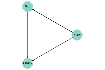
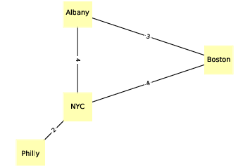
To most people a “graph" is a visual representation of data, like a bar chart or a plot of stock prices over time. That’s not what this chapter is about. In this chapter, a graph is a representation of a system that contains discrete, interconnected elements. The elements are represented by nodes — also called vertices – and the interconnections are represented by edges. For example, you could represent a road map with a node for each city and an edge for each road between cities. Or you could represent a social network using a node for each person, with an edge between two people if they are friends. In some graphs, edges have attributes like length, cost, or weight. For example, in a road map, the length of an edge might represent distance between cities or travel time. In a social network there might be different kinds of edges to represent different kinds of relationships: friends, business associates, etc. Edges may be directed or undirected, depending on whether the relationships they represent are asymmetric or symmetric. In a road map, you might represent a one-way street with a directed edge and a two-way street with an undirected edge. In some social networks, like Facebook, friendship is symmetric: if A is friends with B then B is friends with A. But on Twitter, for example, the “follows” relationship is not symmetric; if A follows B, that doesn’t imply that B follows A. So you might use undirected edges to represent a Facebook network and directed edges for Twitter. Graphs have interesting mathematical properties, and there is a branch of mathematics called graph theory that studies them. Graphs are also useful, because there are many real world problems that can be solved using graph algorithms. For example, Dijkstra’s shortest path algorithm is an efficient way to find the shortest path from a node to all other nodes in a graph. A path is a sequence of nodes with an edge between each consecutive pair. Graphs are usually drawn with squares or circles for nodes and lines for edges. For example, the directed graph in Figure ?? might represent three people who follow each other on Twitter. The arrow indicates the direction of the relationship. In this example, Alice and Bob follow each other, both follow Chuck, and Chuck follows no one. The undirected graph in Figure ?? shows four cities in the northeast United States; the labels on the edges indicate driving time in hours. In this example the placement of the nodes corresponds roughly to the geography of the cities, but in general the layout of a graph is arbitrary. 2.2 NetworkX
To represent graphs, we’ll use a package called NetworkX, which is the most commonly used network library in Python. You can read more about it at http://thinkcomplex.com/netx, but I’ll explain it as we go along. We can create a directed graph by importing NetworkX (usually imported as
At this point,
Now we can use the
The Adding edges works pretty much the same way:
And we can use
NetworkX provides several functions for drawing graphs;
That’s the code I use to generate Figure ??.
The option To generate Figure ??, I start with a dictionary that maps from each city name to its approximate longitude and latitude:
Since this is an undirected graph, I instantiate
Then I can use
Next I’ll make a dictionary that maps from each edge to the corresponding driving time:
Now I can use
Instead of
To add the edge labels, we use
The In both of these examples, the nodes are strings, but in general they can be any hashable type. 2.3 Random graphsA random graph is just what it sounds like: a graph with nodes and edges generated at random. Of course, there are many random processes that can generate graphs, so there are many kinds of random graphs. One of the more interesting kinds is the Erdős-Rényi model, studied by Paul Erdős and Alfréd Rényi in the 1960s. An Erdős-Rényi graph (ER graph) is characterized by two parameters: n is the number of nodes and p is the probability that there is an edge between any two nodes. See http://thinkcomplex.com/er. Erdős and Rényi studied the properties of these random graphs; one of their surprising results is the existence of abrupt changes in the properties of random graphs as random edges are added. One of the properties that displays this kind of transition is connectivity. An undirected graph is connected if there is a path from every node to every other node. In an ER graph, the probability that the graph is connected is very low when p is small and nearly 1 when p is large. Between these two regimes, there is a rapid transition at a particular value of p, denoted p*. Erdős and Rényi showed that this critical value is p* = (lnn) / n, where n is the number of nodes. A random graph, G(n, p), is unlikely to be connected if p < p* and very likely to be connected if p > p*. To test this claim, we’ll develop algorithms to generate random graphs and check whether they are connected. 2.4 Generating graphs
I’ll start by generating a complete graph, which is a graph where every node is connected to every other. Here’s a generator function that takes a list of nodes and enumerates all distinct pairs. If you are not familiar with generator functions, you can read about them at http://thinkcomplex.com/gen.
We can use
The following code makes a complete graph with 10 nodes and draws it:
Figure ?? shows the result. Soon we will modify this code to generate ER graphs, but first we’ll develop functions to check whether a graph is connected. 2.5 Connected graphsA graph is connected if there is a path from every node to every other node (see http://thinkcomplex.com/conn). For many applications involving graphs, it is useful to check whether a graph is connected. Fortunately, there is a simple algorithm that does it. You can start at any node and check whether you can reach all other nodes. If you can reach a node, v, you can reach any of the neighbors of v, which are the nodes connected to v by an edge. The
Suppose we start at node s. We can mark s as “seen” and mark its neighbors. Then we mark the neighbor’s neighbors, and their neighbors, and so on, until we can’t reach any more nodes. If all nodes are seen, the graph is connected. Here’s what that looks like in Python:
Initially the set, Now, each time through the loop, we:
When the stack is empty, we can’t reach any more nodes, so we
break out of the loop and return As an example, we can find all nodes in the complete graph that are reachable from node 0:
Initially, the stack contains node 0 and The next time through the loop, Notice that the same node can appear more than once in the stack; in fact, a node with k neighbors will be added to the stack k times. Later, we will look for ways to make this algorithm more efficient. We can use
A complete graph is, not surprisingly, connected:
In the next section we will generate ER graphs and check whether they are connected. 2.6 Generating ER graphs
The ER graph G(n, p) contains n nodes, and each pair of nodes is connected by an edge with probability p. Generating an ER graph is similar to generating a complete graph. The following generator function enumerates all possible edges and chooses which ones should be added to the graph:
This is the first example we’re seen that uses NumPy. Following convention, I
import So Finally,
Here’s an example with
Figure ?? shows the result. This graph turns out to be connected; in fact, most ER graphs with n=10 and p=0.3 are connected. In the next section, we’ll see how many. 2.7 Probability of connectivity
For given values of n and p, we would like to know the probability that G(n, p) is connected. We can estimate it by generating a large number of random graphs and counting how many are connected. Here’s how:
The parameters This function uses a list comprehension; if you are not familiar with this feature, you can read about it at http://thinkcomplex.com/comp. The result,
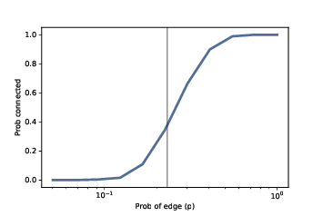
I chose 0.23 because it is close to the critical value where the probability of connectivity goes from near 0 to near 1. According to Erdős and Rényi, p* = lnn / n = 0.23. We can get a clearer view of the transition by estimating the probability of connectivity for a range of values of p:
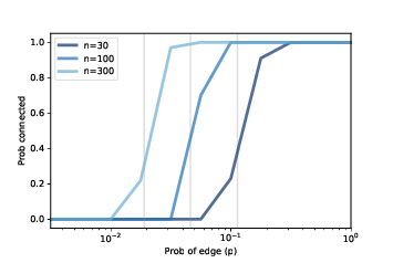
The NumPy function For each value of Figure ?? shows the results, with a vertical line at the computed critical value, p* = 0.23. As expected, the transition from 0 to 1 occurs near the critical value. Figure ?? shows similar results for larger values of n. As n increases, the critical value gets smaller and the transition gets more abrupt. These experimental results are consistent with the analytic results Erdős and Rényi presented in their papers. 2.8 Analysis of graph algorithmsEarlier in this chapter I presented an algorithm for checking whether a graph is connected; in the next few chapters, we will see other graph algorithms. Along the way, we will analyze the performance of those algorithms, figuring out how their run times grow as the size of the graphs increases. If you are not already familiar with analysis of algorithms, you might want to read Appendix B of Think Python, 2nd Edition, at http://thinkcomplex.com/tp2. The order of growth for graph algorithms is usually expressed as a function of n, the number of vertices (nodes), and m, the number of edges. As an example, let’s analyze
Each time through the loop, we pop a node off the stack; by default,
Next we check whether the node is in If the node is not already in To express the run time in terms of n and m, we can add up
the total number of times each node is added to Each node is only added to But nodes might be added to So the total number
of additions to Therefore, the order of growth for this function is O(n + m), which is a convenient way to say that the run time grows in proportion to either n or m, whichever is bigger. If we know the relationship between n and m, we can simplify
this expression. For example, in a complete graph the number of edges
is n(n−1)/2, which is in O(n2). So for a complete graph,
2.9 ExercisesThe code for this chapter is in Exercise 1
Launch chap02.ipynb and run the code. There are a few short
exercises embedded in the notebook that you might want to try.
Exercise 2
In Section ?? we analyzed the performance of
reachable_nodes and classified it in O(n + m), where n is the
number of nodes and m is the number of edges. Continuing the
analysis, what is the order of growth for is_connected?
Exercise 3
In my implementation of reachable_nodes, you might be bothered by
the apparent inefficiency of adding all neighbors to the stack
without checking whether they are already in seen. Write a
version of this function that checks the neighbors before adding them
to the stack. Does this “optimization” change the order of growth?
Does it make the function faster?
Exercise 4
There are actually two kinds of ER graphs. The one we generated in this chapter, G(n, p), is characterized by two parameters, the number of nodes and the probability of an edge between nodes. An alternative definition, denoted G(n, m), is also characterized by two parameters: the number of nodes, n, and the number of edges, m. Under this definition, the number of edges is fixed, but their location is random. Repeat the experiments we did in this chapter using this alternative definition. Here are a few suggestions for how to proceed: 1. Write a function called 2. Write a function called 3. Make a version of 4. Compute the probability of connectivity for a range of values of m. How do the results of this experiment compare to the results using the first type of ER graph? |
Buy this book at Amazon.com
ContributeIf you would like to make a contribution to support my books, you can use the button below and pay with PayPal. Thank you!
Are you using one of our books in a class?We'd like to know about it. Please consider filling out this short survey.
|